敏感性分析示例
方法
我们提供了五种敏感性分析方法,包括(安慰剂处理、随机原因、子集数据、随机替换和选择偏差)。本笔记本将逐步介绍如何使用组合函数 sensitivity_analysis() 来比较不同的方法,以及如何单独使用每种方法:
安慰剂处理:用随机变量替换处理
无关的额外混杂因素:添加一个随机共同原因变量
子集验证:移除数据的随机子集
选择偏差方法,包括单边混淆函数和对齐混淆函数
随机替换:随机将一个协变量替换为一个不相关的变量
[2]:
%matplotlib inline
%load_ext autoreload
%autoreload 2
[3]:
import pandas as pd
import matplotlib.pyplot as plt
from sklearn.linear_model import LinearRegression
import warnings
import matplotlib
from causalml.inference.meta import BaseXLearner
from causalml.dataset import synthetic_data

from causalml.metrics.sensitivity import Sensitivity
from causalml.metrics.sensitivity import SensitivityRandomReplace, SensitivitySelectionBias

plt.style.use('fivethirtyeight')
matplotlib.rcParams['figure.figsize'] = [8, 8]
warnings.filterwarnings('ignore')

# logging.basicConfig(level=logging.INFO)

pd.options.display.float_format = '{:.4f}'.format
/Users/jing.pan/anaconda3/envs/causalml_3_6/lib/python3.6/site-packages/sklearn/utils/deprecation.py:144: FutureWarning: The sklearn.utils.testing module is  deprecated in version 0.22 and will be removed in version 0.24. The corresponding classes / functions should instead be imported from sklearn.utils. Anything that cannot be imported from sklearn.utils is now part of the private API.
  warnings.warn(message, FutureWarning)
生成合成数据
[4]:
# Generate synthetic data using mode 1
num_features = 6
y, X, treatment, tau, b, e = synthetic_data(mode=1, n=100000, p=num_features, sigma=1.0)
[5]:
tau.mean()
[5]:
0.5001096146567363
定义特征
[6]:
# Generate features names
INFERENCE_FEATURES = ['feature_' + str(i) for i in range(num_features)]
TREATMENT_COL = 'target'
OUTCOME_COL = 'outcome'
SCORE_COL = 'pihat'
[7]:
df = pd.DataFrame(X, columns=INFERENCE_FEATURES)
df[TREATMENT_COL] = treatment
df[OUTCOME_COL] = y
df[SCORE_COL] = e
[8]:
df.head()
[8]:
| 特征_0 | 特征_1 | 特征_2 | 特征_3 | 特征_4 | 特征_5 | 目标 | 结果 | pihat | |
|---|---|---|---|---|---|---|---|---|---|
| 0 | 0.9536 | 0.2911 | 0.0432 | 0.8720 | 0.5190 | 0.0822 | 1 | 2.0220 | 0.7657 |
| 1 | 0.2390 | 0.3096 | 0.5115 | 0.2048 | 0.8914 | 0.5015 | 0 | -0.0732 | 0.2304 |
| 2 | 0.1091 | 0.0765 | 0.7428 | 0.6951 | 0.4580 | 0.7800 | 0 | -1.4947 | 0.1000 |
| 3 | 0.2055 | 0.3967 | 0.6278 | 0.2086 | 0.3865 | 0.8860 | 0 | 0.6458 | 0.2533 |
| 4 | 0.4501 | 0.0578 | 0.3972 | 0.4100 | 0.5760 | 0.4764 | 0 | -0.0018 | 0.1000 |
包含所有协变量
敏感性分析总结报告(使用单侧混杂函数和默认alpha值)
[9]:
# Calling the Base XLearner class and return the sensitivity analysis summary report
learner_x = BaseXLearner(LinearRegression())
sens_x = Sensitivity(df=df, inference_features=INFERENCE_FEATURES, p_col='pihat',
                     treatment_col=TREATMENT_COL, outcome_col=OUTCOME_COL, learner=learner_x)
# Here for Selection Bias method will use default one-sided confounding function and alpha (quantile range of outcome values) input
sens_sumary_x = sens_x.sensitivity_analysis(methods=['Placebo Treatment',
                                                     'Random Cause',
                                                     'Subset Data',
                                                     'Random Replace',
                                                     'Selection Bias'], sample_size=0.5)
[10]:
# From the following results, refutation methods show our model is pretty robust;
# When alpah > 0, the treated group always has higher mean potential outcomes than the control; when  < 0, the control group is better off.
sens_sumary_x
[10]:
| 方法 | ATE | 新ATE | 新ATE下限 | 新ATE上限 | |
|---|---|---|---|---|---|
| 0 | 安慰剂治疗 | 0.6801 | -0.0025 | -0.0158 | 0.0107 |
| 0 | 随机原因 | 0.6801 | 0.6801 | 0.6673 | 0.6929 |
| 0 | 子集数据(样本大小 @0.5) | 0.6801 | 0.6874 | 0.6693 | 0.7055 |
| 0 | 随机替换 | 0.6801 | 0.6799 | 0.6670 | 0.6929 |
| 0 | 选择偏差 (alpha@-0.80111, 具有 r-平方:... | 0.6801 | 1.3473 | 1.3347 | 1.3599 |
| 0 | 选择偏差 (alpha@-0.64088, 与 r-平方:... | 0.6801 | 1.2139 | 1.2013 | 1.2265 |
| 0 | 选择偏差 (alpha@-0.48066, 具有 r-平方:... | 0.6801 | 1.0804 | 1.0678 | 1.0931 |
| 0 | 选择偏差 (alpha@-0.32044, 具有 r-平方:... | 0.6801 | 0.9470 | 0.9343 | 0.9597 |
| 0 | 选择偏差 (alpha@-0.16022, 具有 r-平方:... | 0.6801 | 0.8135 | 0.8008 | 0.8263 |
| 0 | 选择偏差 (alpha@0.0, 具有 r-平方:0.0 | 0.6801 | 0.6801 | 0.6673 | 0.6929 |
| 0 | 选择偏差 (alpha@0.16022, 与 r-平方:0... | 0.6801 | 0.5467 | 0.5338 | 0.5595 |
| 0 | 选择偏差 (alpha@0.32044, 带有 r-平方:0... | 0.6801 | 0.4132 | 0.4003 | 0.4261 |
| 0 | 选择偏差 (alpha@0.48066, 具有 r-平方:0... | 0.6801 | 0.2798 | 0.2668 | 0.2928 |
| 0 | 选择偏差 (alpha@0.64088, 具有 r-平方:0... | 0.6801 | 0.1463 | 0.1332 | 0.1594 |
| 0 | 选择偏差 (alpha@0.80111, 具有 r-平方:0... | 0.6801 | 0.0129 | -0.0003 | 0.0261 |
随机替换
[11]:
# Replace feature_0 with an irrelevent variable
sens_x_replace = SensitivityRandomReplace(df=df, inference_features=INFERENCE_FEATURES, p_col='pihat',
                                          treatment_col=TREATMENT_COL, outcome_col=OUTCOME_COL, learner=learner_x,
                                          sample_size=0.9, replaced_feature='feature_0')
s_check_replace = sens_x_replace.summary(method='Random Replace')
s_check_replace
[11]:
| 方法 | ATE | 新ATE | 新ATE下限 | 新ATE上限 | |
|---|---|---|---|---|---|
| 0 | 随机替换 | 0.6801 | 0.8072 | 0.7943 | 0.8200 |
选择偏差:对齐混淆函数
[12]:
sens_x_bias_alignment = SensitivitySelectionBias(df, INFERENCE_FEATURES, p_col='pihat', treatment_col=TREATMENT_COL,
                                                 outcome_col=OUTCOME_COL, learner=learner_x, confound='alignment',
                                                 alpha_range=None)
[13]:
lls_x_bias_alignment, partial_rsqs_x_bias_alignment = sens_x_bias_alignment.causalsens()
[14]:
lls_x_bias_alignment
[14]:
| alpha | rsqs | 新ATE | 新ATE下限 | 新ATE上限 | |
|---|---|---|---|---|---|
| 0 | -0.8011 | 0.1088 | 0.6685 | 0.6556 | 0.6813 |
| 0 | -0.6409 | 0.0728 | 0.6708 | 0.6580 | 0.6836 |
| 0 | -0.4807 | 0.0425 | 0.6731 | 0.6604 | 0.6859 |
| 0 | -0.3204 | 0.0194 | 0.6754 | 0.6627 | 0.6882 |
| 0 | -0.1602 | 0.0050 | 0.6778 | 0.6650 | 0.6905 |
| 0 | 0.0000 | 0.0000 | 0.6801 | 0.6673 | 0.6929 |
| 0 | 0.1602 | 0.0050 | 0.6824 | 0.6696 | 0.6953 |
| 0 | 0.3204 | 0.0200 | 0.6848 | 0.6718 | 0.6977 |
| 0 | 0.4807 | 0.0443 | 0.6871 | 0.6741 | 0.7001 |
| 0 | 0.6409 | 0.0769 | 0.6894 | 0.6763 | 0.7026 |
| 0 | 0.8011 | 0.1164 | 0.6918 | 0.6785 | 0.7050 |
[15]:
partial_rsqs_x_bias_alignment
[15]:
| 特征 | 部分_rsqs | |
|---|---|---|
| 0 | feature_0 | -0.0631 |
| 1 | feature_1 | -0.0619 |
| 2 | feature_2 | -0.0001 |
| 3 | feature_3 | -0.0033 |
| 4 | feature_4 | -0.0001 |
| 5 | feature_5 | 0.0000 |
[16]:
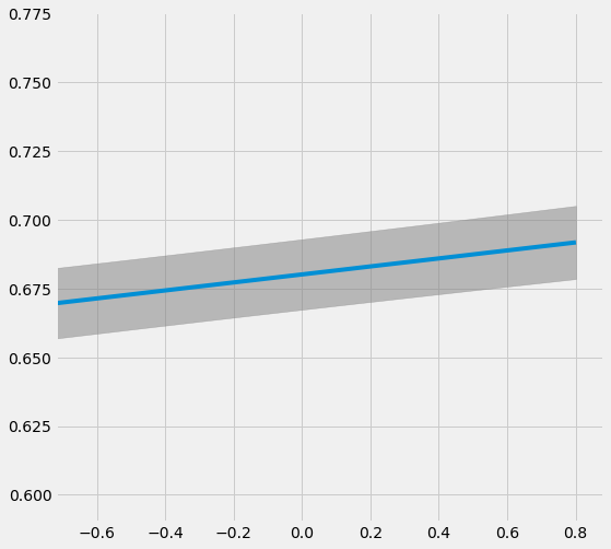
# Plot the results by confounding vector and plot Confidence Intervals for ATE
sens_x_bias_alignment.plot(lls_x_bias_alignment, ci=True)
[17]:
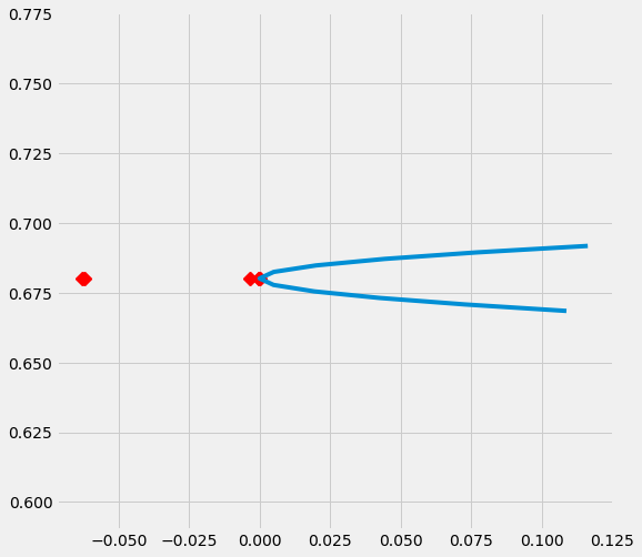
# Plot the results by rsquare with partial r-square results by each individual features
sens_x_bias_alignment.plot(lls_x_bias_alignment, partial_rsqs_x_bias_alignment, type='r.squared', partial_rsqs=True)
删除一个混淆变量
[18]:
df_new = df.drop('feature_0', axis=1).copy()
INFERENCE_FEATURES_new = INFERENCE_FEATURES.copy()
INFERENCE_FEATURES_new.remove('feature_0')
df_new.head()
[18]:
| 特征_1 | 特征_2 | 特征_3 | 特征_4 | 特征_5 | 目标 | 结果 | pihat | |
|---|---|---|---|---|---|---|---|---|
| 0 | 0.2911 | 0.0432 | 0.8720 | 0.5190 | 0.0822 | 1 | 2.0220 | 0.7657 |
| 1 | 0.3096 | 0.5115 | 0.2048 | 0.8914 | 0.5015 | 0 | -0.0732 | 0.2304 |
| 2 | 0.0765 | 0.7428 | 0.6951 | 0.4580 | 0.7800 | 0 | -1.4947 | 0.1000 |
| 3 | 0.3967 | 0.6278 | 0.2086 | 0.3865 | 0.8860 | 0 | 0.6458 | 0.2533 |
| 4 | 0.0578 | 0.3972 | 0.4100 | 0.5760 | 0.4764 | 0 | -0.0018 | 0.1000 |
[19]:
INFERENCE_FEATURES_new
[19]:
['feature_1', 'feature_2', 'feature_3', 'feature_4', 'feature_5']
敏感性分析总结报告(使用单侧混杂函数和默认alpha值)
[20]:
sens_x_new = Sensitivity(df=df_new, inference_features=INFERENCE_FEATURES_new, p_col='pihat',
                     treatment_col=TREATMENT_COL, outcome_col=OUTCOME_COL, learner=learner_x)
# Here for Selection Bias method will use default one-sided confounding function and alpha (quantile range of outcome values) input
sens_sumary_x_new = sens_x_new.sensitivity_analysis(methods=['Placebo Treatment',
                                                     'Random Cause',
                                                     'Subset Data',
                                                     'Random Replace',
                                                     'Selection Bias'], sample_size=0.5)
[21]:
# Here we can see the New ATE restul from Random Replace method actually changed ~ 12.5%
sens_sumary_x_new
[21]:
| 方法 | ATE | 新ATE | 新ATE下限 | 新ATE上限 | |
|---|---|---|---|---|---|
| 0 | 安慰剂治疗 | 0.8072 | 0.0104 | -0.0033 | 0.0242 |
| 0 | 随机原因 | 0.8072 | 0.8072 | 0.7943 | 0.8201 |
| 0 | 子集数据(样本大小 @0.5) | 0.8072 | 0.8180 | 0.7998 | 0.8361 |
| 0 | 随机替换 | 0.8072 | 0.8068 | 0.7938 | 0.8198 |
| 0 | 选择偏差 (alpha@-0.80111, 与 r-平方:... | 0.8072 | 1.3799 | 1.3673 | 1.3925 |
| 0 | 选择偏差 (alpha@-0.64088, 与 r-平方:... | 0.8072 | 1.2654 | 1.2527 | 1.2780 |
| 0 | 选择偏差 (alpha@-0.48066, 具有 r-平方:... | 0.8072 | 1.1508 | 1.1381 | 1.1635 |
| 0 | 选择偏差 (alpha@-0.32044, 具有 r-平方:... | 0.8072 | 1.0363 | 1.0235 | 1.0490 |
| 0 | 选择偏差 (alpha@-0.16022, 与 r-平方:... | 0.8072 | 0.9217 | 0.9089 | 0.9345 |
| 0 | 选择偏差 (alpha@0.0, 带有 r-平方:0.0 | 0.8072 | 0.8072 | 0.7943 | 0.8200 |
| 0 | 选择偏差 (alpha@0.16022, 与 r-平方:0... | 0.8072 | 0.6926 | 0.6796 | 0.7056 |
| 0 | 选择偏差 (alpha@0.32044, 具有 r-平方:0... | 0.8072 | 0.5780 | 0.5650 | 0.5911 |
| 0 | 选择偏差 (alpha@0.48066, 具有 r-平方:0... | 0.8072 | 0.4635 | 0.4503 | 0.4767 |
| 0 | 选择偏差 (alpha@0.64088, 与 r-平方:0... | 0.8072 | 0.3489 | 0.3356 | 0.3623 |
| 0 | 选择偏差 (alpha@0.80111, 具有 r-平方:0... | 0.8072 | 0.2344 | 0.2209 | 0.2479 |
随机替换
[22]:
# Replace feature_0 with an irrelevent variable
sens_x_replace_new = SensitivityRandomReplace(df=df_new, inference_features=INFERENCE_FEATURES_new, p_col='pihat',
                                          treatment_col=TREATMENT_COL, outcome_col=OUTCOME_COL, learner=learner_x,
                                          sample_size=0.9, replaced_feature='feature_1')
s_check_replace_new = sens_x_replace_new.summary(method='Random Replace')
s_check_replace_new
[22]:
| 方法 | ATE | 新ATE | 新ATE下限 | 新ATE上限 | |
|---|---|---|---|---|---|
| 0 | 随机替换 | 0.8072 | 0.9022 | 0.8893 | 0.9152 |
选择偏差:对齐混淆函数
[23]:
sens_x_bias_alignment_new = SensitivitySelectionBias(df_new, INFERENCE_FEATURES_new, p_col='pihat', treatment_col=TREATMENT_COL,
                                                 outcome_col=OUTCOME_COL, learner=learner_x, confound='alignment',
                                                 alpha_range=None)
[24]:
lls_x_bias_alignment_new, partial_rsqs_x_bias_alignment_new = sens_x_bias_alignment_new.causalsens()
[25]:
lls_x_bias_alignment_new
[25]:
| alpha | rsqs | 新ATE | 新ATE下限 | 新ATE上限 | |
|---|---|---|---|---|---|
| 0 | -0.8011 | 0.1121 | 0.7919 | 0.7789 | 0.8049 |
| 0 | -0.6409 | 0.0732 | 0.7950 | 0.7820 | 0.8079 |
| 0 | -0.4807 | 0.0419 | 0.7980 | 0.7851 | 0.8109 |
| 0 | -0.3204 | 0.0188 | 0.8011 | 0.7882 | 0.8139 |
| 0 | -0.1602 | 0.0047 | 0.8041 | 0.7912 | 0.8170 |
| 0 | 0.0000 | 0.0000 | 0.8072 | 0.7943 | 0.8200 |
| 0 | 0.1602 | 0.0048 | 0.8102 | 0.7973 | 0.8231 |
| 0 | 0.3204 | 0.0189 | 0.8133 | 0.8003 | 0.8262 |
| 0 | 0.4807 | 0.0420 | 0.8163 | 0.8032 | 0.8294 |
| 0 | 0.6409 | 0.0736 | 0.8194 | 0.8062 | 0.8325 |
| 0 | 0.8011 | 0.1127 | 0.8224 | 0.8091 | 0.8357 |
[26]:
partial_rsqs_x_bias_alignment_new
[26]:
| 特征 | 部分_rsqs | |
|---|---|---|
| 0 | feature_1 | -0.0345 |
| 1 | feature_2 | -0.0001 |
| 2 | feature_3 | -0.0038 |
| 3 | feature_4 | -0.0001 |
| 4 | feature_5 | 0.0000 |
[27]:
# Plot the results by confounding vector and plot Confidence Intervals for ATE
sens_x_bias_alignment_new.plot(lls_x_bias_alignment_new, ci=True)

[28]:
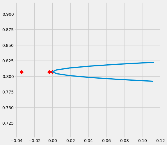
# Plot the results by rsquare with partial r-square results by each individual features
sens_x_bias_alignment_new.plot(lls_x_bias_alignment_new, partial_rsqs_x_bias_alignment_new, type='r.squared', partial_rsqs=True)
生成一个选择偏差集
[29]:
df_new_2 = df.copy()
df_new_2['treated_new'] = df['feature_0'].rank()
df_new_2['treated_new'] = [1 if i > df_new_2.shape[0]/2 else 0 for i in df_new_2['treated_new']]
[30]:
df_new_2.head()
[30]:
| 特征_0 | 特征_1 | 特征_2 | 特征_3 | 特征_4 | 特征_5 | 目标 | 结果 | pihat | treated_new | |
|---|---|---|---|---|---|---|---|---|---|---|
| 0 | 0.9536 | 0.2911 | 0.0432 | 0.8720 | 0.5190 | 0.0822 | 1 | 2.0220 | 0.7657 | 1 |
| 1 | 0.2390 | 0.3096 | 0.5115 | 0.2048 | 0.8914 | 0.5015 | 0 | -0.0732 | 0.2304 | 0 |
| 2 | 0.1091 | 0.0765 | 0.7428 | 0.6951 | 0.4580 | 0.7800 | 0 | -1.4947 | 0.1000 | 0 |
| 3 | 0.2055 | 0.3967 | 0.6278 | 0.2086 | 0.3865 | 0.8860 | 0 | 0.6458 | 0.2533 | 0 |
| 4 | 0.4501 | 0.0578 | 0.3972 | 0.4100 | 0.5760 | 0.4764 | 0 | -0.0018 | 0.1000 | 0 |
敏感性分析总结报告(使用单侧混杂函数和默认alpha值)
[31]:
sens_x_new_2 = Sensitivity(df=df_new_2, inference_features=INFERENCE_FEATURES, p_col='pihat',
                     treatment_col='treated_new', outcome_col=OUTCOME_COL, learner=learner_x)
# Here for Selection Bias method will use default one-sided confounding function and alpha (quantile range of outcome values) input
sens_sumary_x_new_2 = sens_x_new_2.sensitivity_analysis(methods=['Placebo Treatment',
                                                     'Random Cause',
                                                     'Subset Data',
                                                     'Random Replace',
                                                     'Selection Bias'], sample_size=0.5)
[32]:
sens_sumary_x_new_2
[32]:
| 方法 | ATE | 新ATE | 新ATE下限 | 新ATE上限 | |
|---|---|---|---|---|---|
| 0 | 安慰剂治疗 | 0.0432 | 0.0081 | -0.0052 | 0.0213 |
| 0 | 随机原因 | 0.0432 | 0.0432 | 0.0296 | 0.0568 |
| 0 | 子集数据(样本大小 @0.5) | 0.0432 | 0.0976 | 0.0784 | 0.1167 |
| 0 | 随机替换 | 0.0432 | 0.0433 | 0.0297 | 0.0568 |
| 0 | 选择偏差 (alpha@-0.80111, 具有 r-平方:... | 0.0432 | 0.8369 | 0.8239 | 0.8499 |
| 0 | 选择偏差 (alpha@-0.64088, 与 r-平方:... | 0.0432 | 0.6782 | 0.6651 | 0.6913 |
| 0 | 选择偏差 (alpha@-0.48066, 具有 r-平方:... | 0.0432 | 0.5194 | 0.5063 | 0.5326 |
| 0 | 选择偏差 (alpha@-0.32044, 具有 r-平方:... | 0.0432 | 0.3607 | 0.3474 | 0.3740 |
| 0 | 选择偏差 (alpha@-0.16022, 具有 r-平方:... | 0.0432 | 0.2020 | 0.1885 | 0.2154 |
| 0 | 选择偏差 (alpha@0.0, 带有 r-平方:0.0 | 0.0432 | 0.0432 | 0.0296 | 0.0568 |
| 0 | 选择偏差 (alpha@0.16022, 具有 r-平方:0... | 0.0432 | -0.1155 | -0.1293 | -0.1018 |
| 0 | 选择偏差 (alpha@0.32044, 具有 r-平方:0... | 0.0432 | -0.2743 | -0.2882 | -0.2604 |
| 0 | 选择偏差 (alpha@0.48066, 具有 r-平方:0... | 0.0432 | -0.4330 | -0.4471 | -0.4189 |
| 0 | 选择偏差 (alpha@0.64088, 具有 r-平方:0... | 0.0432 | -0.5918 | -0.6060 | -0.5775 |
| 0 | 选择偏差 (alpha@0.80111, 具有 r-平方:0... | 0.0432 | -0.7505 | -0.7650 | -0.7360 |
随机替换
[33]:
# Replace feature_0 with an irrelevent variable
sens_x_replace_new_2 = SensitivityRandomReplace(df=df_new_2, inference_features=INFERENCE_FEATURES, p_col='pihat',
                                          treatment_col='treated_new', outcome_col=OUTCOME_COL, learner=learner_x,
                                          sample_size=0.9, replaced_feature='feature_0')
s_check_replace_new_2 = sens_x_replace_new_2.summary(method='Random Replace')
s_check_replace_new_2
[33]:
| 方法 | ATE | 新ATE | 新ATE下限 | 新ATE上限 | |
|---|---|---|---|---|---|
| 0 | 随机替换 | 0.0432 | 0.4847 | 0.4713 | 0.4981 |
选择偏差:对齐混淆函数
[34]:
sens_x_bias_alignment_new_2 = SensitivitySelectionBias(df_new_2, INFERENCE_FEATURES, p_col='pihat', treatment_col='treated_new',
                                                 outcome_col=OUTCOME_COL, learner=learner_x, confound='alignment',
                                                 alpha_range=None)
[35]:
lls_x_bias_alignment_new_2, partial_rsqs_x_bias_alignment_new_2 = sens_x_bias_alignment_new_2.causalsens()
[36]:
lls_x_bias_alignment_new_2
[36]:
| alpha | rsqs | 新ATE | 新ATE下限 | 新ATE上限 | |
|---|---|---|---|---|---|
| 0 | -0.8011 | 0.0604 | -0.2260 | -0.2399 | -0.2120 |
| 0 | -0.6409 | 0.0415 | -0.1721 | -0.1860 | -0.1583 |
| 0 | -0.4807 | 0.0250 | -0.1183 | -0.1320 | -0.1045 |
| 0 | -0.3204 | 0.0119 | -0.0645 | -0.0781 | -0.0508 |
| 0 | -0.1602 | 0.0032 | -0.0106 | -0.0242 | 0.0030 |
| 0 | 0.0000 | 0.0000 | 0.0432 | 0.0296 | 0.0568 |
| 0 | 0.1602 | 0.0035 | 0.0971 | 0.0835 | 0.1106 |
| 0 | 0.3204 | 0.0148 | 0.1509 | 0.1373 | 0.1645 |
| 0 | 0.4807 | 0.0347 | 0.2047 | 0.1911 | 0.2183 |
| 0 | 0.6409 | 0.0635 | 0.2586 | 0.2449 | 0.2722 |
| 0 | 0.8011 | 0.1013 | 0.3124 | 0.2986 | 0.3262 |
[37]:
partial_rsqs_x_bias_alignment_new_2
[37]:
| 特征 | 部分_rsqs | |
|---|---|---|
| 0 | feature_0 | -0.4041 |
| 1 | feature_1 | 0.0101 |
| 2 | feature_2 | 0.0000 |
| 3 | feature_3 | 0.0016 |
| 4 | feature_4 | 0.0011 |
| 5 | feature_5 | 0.0000 |
[38]:
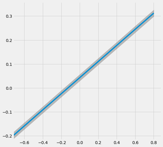
# Plot the results by confounding vector and plot Confidence Intervals for ATE
sens_x_bias_alignment_new_2.plot(lls_x_bias_alignment_new_2, ci=True)
[39]:
# Plot the results by rsquare with partial r-square results by each individual features
sens_x_bias_alignment_new_2.plot(lls_x_bias_alignment_new, partial_rsqs_x_bias_alignment_new_2, type='r.squared', partial_rsqs=True)
