使用合成数据的提升树示例

在本笔记本中，我们使用合成数据来演示基于树的算法的使用。

[3]:

import numpy as np
import pandas as pd

from causalml.dataset import make_uplift_classification
from causalml.inference.tree import UpliftRandomForestClassifier
from causalml.metrics import plot_gain

from sklearn.model_selection import train_test_split

[4]:

import importlib
print(importlib.metadata.version('causalml') )

0.14.0

生成合成数据集

CausalML 包包含各种函数，用于生成用于提升建模的合成数据集。在这里，我们使用 make_uplift_classification() 函数生成一个分类数据集。

[3]:

df, x_names = make_uplift_classification()

[4]:

df.head()

[4]:

	treatment_group_key	x1_informative	x2_informative	x3_informative	x4_informative	x5_informative	x6_irrelevant	x7_irrelevant	x8_irrelevant	x9_irrelevant	...	x12_uplift_increase	x13_increase_mix	x14_uplift_increase	x15_uplift_increase	x16_increase_mix	x17_uplift_increase	x18_uplift_increase	x19_increase_mix	conversion	treatment_effect
0	control	-0.542888	1.976361	-0.531359	-2.354211	-0.380629	-2.614321	-0.128893	0.448689	-2.275192	...	-1.315304	0.742654	1.891699	-2.428395	1.541875	-0.817705	-0.610194	-0.591581	0	0
1	treatment3	0.258654	0.552412	1.434239	-1.422311	0.089131	0.790293	1.159513	1.578868	0.166540	...	-1.391878	-0.623243	2.443972	-2.889253	2.018585	-1.109296	-0.380362	-1.667606	0	0
2	treatment1	1.697012	-2.762600	-0.662874	-1.682340	1.217443	0.837982	1.042981	0.177398	-0.112409	...	-1.132497	1.050179	1.573054	-1.788427	1.341609	-0.749227	-2.091521	-0.471386	0	0
3	treatment2	-1.441644	1.823648	0.789423	-0.295398	0.718509	-0.492993	0.947824	-1.307887	0.123340	...	-2.084619	0.058481	1.369439	0.422538	1.087176	-0.966666	-1.785592	-1.268379	1	1
4	控制	-0.625074	3.002388	-0.096288	1.938235	3.392424	-0.465860	-0.919897	-1.072592	-1.331181	...	-1.403984	0.760430	1.917635	-2.347675	1.560946	-0.833067	-1.407884	-0.781343	0	0

5 行 × 22 列

[5]:

# Look at the conversion rate and sample size in each group
df.pivot_table(values='conversion',
               index='treatment_group_key',
               aggfunc=[np.mean, np.size],
               margins=True)

[5]:

	平均值	大小
	转化	转化
treatment_group_key
控制	0.511	1000
treatment1	0.514	1000
treatment2	0.559	1000
treatment3	0.600	1000
全部	0.546	4000

运行提升随机森林分类器

在本节中，我们首先使用训练数据拟合提升随机森林分类器。然后，我们使用拟合的模型对测试数据进行预测。预测返回一个ndarray，其中每列包含如果单位在相应的处理组中时的预测提升。

[6]:

# Split data to training and testing samples for model validation (next section)
df_train, df_test = train_test_split(df, test_size=0.2, random_state=111)

[7]:

from causalml.inference.tree import UpliftTreeClassifier

[8]:

clf = UpliftTreeClassifier(control_name='control')
clf.fit(df_train[x_names].values,
         treatment=df_train['treatment_group_key'].values,
         y=df_train['conversion'].values)
p = clf.predict(df_test[x_names].values)

[9]:

df_res = pd.DataFrame(p, columns=clf.classes_)
df_res.head()

[9]:

	控制组	处理组1	处理组2	处理组3
0	0.506394	0.511811	0.573935	0.503778
1	0.506394	0.511811	0.573935	0.503778
2	0.580838	0.458824	0.508982	0.452381
3	0.482558	0.572327	0.556757	0.961538
4	0.482558	0.572327	0.556757	0.961538

[10]:

uplift_model = UpliftRandomForestClassifier(control_name='control')

[11]:

uplift_model.fit(df_train[x_names].values,
                 treatment=df_train['treatment_group_key'].values,
                 y=df_train['conversion'].values)

[12]:

df_res = uplift_model.predict(df_test[x_names].values, full_output=True)
print(df_res.shape)
df_res.head()

(800, 9)

[12]:

	控制组	处理组1	处理组2	处理组3	推荐处理	处理组1差异	处理组2差异	处理组3差异	最大差异
0	0.415263	0.401823	0.465554	0.391658	2	-0.013440	0.050291	-0.023605	0.050291
1	0.412962	0.389346	0.476169	0.363343	2	-0.023616	0.063206	-0.049619	0.063206
2	0.533442	0.548670	0.589756	0.588654	2	0.015228	0.056313	0.055212	0.056313
3	0.344854	0.314433	0.370315	0.760676	3	-0.030420	0.025461	0.415822	0.415822
4	0.649657	0.602642	0.641364	0.851301	3	-0.047015	-0.008293	0.201644	0.201644

[13]:

y_pred = uplift_model.predict(df_test[x_names].values)

[14]:

y_pred.shape

[14]:

(800, 3)

[15]:

# Put the predictions to a DataFrame for a neater presentation
# The output of `predict()` is a numpy array with the shape of [n_sample, n_treatment] excluding the
# predictions for the control group.
result = pd.DataFrame(y_pred,
                      columns=uplift_model.classes_[1:])
result.head()

[15]:

	处理1	处理2	处理3
0	-0.013440	0.050291	-0.023605
1	-0.023616	0.063206	-0.049619
2	0.015228	0.056313	0.055212
3	-0.030420	0.025461	0.415822
4	-0.047015	-0.008293	0.201644

创建提升曲线

模型的性能可以通过uplift曲线来评估。

创建一个合成人口

提升曲线是在一个合成群体上计算的，该群体包括那些在对照组中的个体和那些恰好被模型推荐到处理组中的个体。我们使用这个合成群体来计算在预测的处理效应分位数内的实际处理效应。由于数据是随机化的，我们在预测的分位数中大致有相等数量的处理组和对照组观察值，并且没有自我选择进入处理组的情况。

[16]:

# If all deltas are negative, assing to control; otherwise assign to the treatment
# with the highest delta
best_treatment = np.where((result < 0).all(axis=1),
                           'control',
                           result.idxmax(axis=1))

# Create indicator variables for whether a unit happened to have the
# recommended treatment or was in the control group
actual_is_best = np.where(df_test['treatment_group_key'] == best_treatment, 1, 0)
actual_is_control = np.where(df_test['treatment_group_key'] == 'control', 1, 0)

[17]:

synthetic = (actual_is_best == 1) | (actual_is_control == 1)
synth = result[synthetic]

计算每个预测治疗效果分位数的观察治疗效果

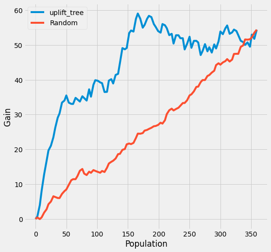
我们使用观察到的治疗效果来计算提升曲线，该曲线回答了以下问题：通过根据预测的提升从高到低排序的人口子集进行定位，我们可以捕获多少总累积提升？

CausalML 具有 plot_gain() 函数，该函数计算给定包含处理分配、观察结果和预测处理效果的 DataFrame 的提升曲线。

[18]:

auuc_metrics = (synth.assign(is_treated = 1 - actual_is_control[synthetic],
                             conversion = df_test.loc[synthetic, 'conversion'].values,
                             uplift_tree = synth.max(axis=1))
                     .drop(columns=list(uplift_model.classes_[1:])))

[19]:

plot_gain(auuc_metrics, outcome_col='conversion', treatment_col='is_treated')

../_images/examples_uplift_trees_with_synthetic_data_24_0.png

[ ]: