使用TMLE示例的提升曲线
本笔记本演示了在不知道真实治疗效果的情况下使用提升曲线的问题,以及如何通过使用TMLE作为真实治疗效果的代理来解决这个问题。
[1]:
%reload_ext autoreload
%autoreload 2
%matplotlib inline
[2]:
import os
base_path = os.path.abspath("../")
os.chdir(base_path)
[3]:
import logging
from matplotlib import pyplot as plt
import numpy as np
import pandas as pd
from sklearn.model_selection import train_test_split, KFold
import sys
import warnings
warnings.simplefilter("ignore", UserWarning)

from lightgbm import LGBMRegressor
[4]:
import causalml

from causalml.dataset import synthetic_data
from causalml.inference.meta import BaseXRegressor, TMLELearner
from causalml.metrics.visualize import *
from causalml.propensity import calibrate

import importlib
print(importlib.metadata.version('causalml') )
Failed to import duecredit due to No module named 'duecredit'
0.15.3.dev0
[5]:
logger = logging.getLogger('causalml')
logger.setLevel(logging.DEBUG)
plt.style.use('fivethirtyeight')
生成合成数据
[6]:
# Generate synthetic data using mode 1
y, X, treatment, tau, b, e = synthetic_data(mode=1, n=1000000, p=10, sigma=5.)
[7]:
X_train, X_test, y_train, y_test, e_train, e_test, treatment_train, treatment_test, tau_train, tau_test, b_train, b_test = train_test_split(X, y, e, treatment, tau, b, test_size=0.5, random_state=42)
计算个体治疗效果 (ITE/CATE)
[8]:
# X Learner
learner_x = BaseXRegressor(learner=LGBMRegressor())
learner_x.fit(X=X_train, treatment=treatment_train, y=y_train)
cate_x_test = learner_x.predict(X=X_test, p=e_test, treatment=treatment_test).flatten()
[LightGBM] [Info] Auto-choosing row-wise multi-threading, the overhead of testing was 0.000981 seconds.
You can set `force_row_wise=true` to remove the overhead.
And if memory is not enough, you can set `force_col_wise=true`.
[LightGBM] [Info] Total Bins 2550
[LightGBM] [Info] Number of data points in the train set: 240455, number of used features: 10
[LightGBM] [Info] Start training from score 1.025470
[LightGBM] [Info] Auto-choosing row-wise multi-threading, the overhead of testing was 0.000968 seconds.
You can set `force_row_wise=true` to remove the overhead.
And if memory is not enough, you can set `force_col_wise=true`.
[LightGBM] [Info] Total Bins 2550
[LightGBM] [Info] Number of data points in the train set: 259545, number of used features: 10
[LightGBM] [Info] Start training from score 1.931372
[LightGBM] [Info] Auto-choosing row-wise multi-threading, the overhead of testing was 0.000901 seconds.
You can set `force_row_wise=true` to remove the overhead.
And if memory is not enough, you can set `force_col_wise=true`.
[LightGBM] [Info] Total Bins 2550
[LightGBM] [Info] Number of data points in the train set: 240455, number of used features: 10
[LightGBM] [Info] Start training from score 0.429150
[LightGBM] [Info] Auto-choosing row-wise multi-threading, the overhead of testing was 0.000983 seconds.
You can set `force_row_wise=true` to remove the overhead.
And if memory is not enough, you can set `force_col_wise=true`.
[LightGBM] [Info] Total Bins 2550
[LightGBM] [Info] Number of data points in the train set: 259545, number of used features: 10
[LightGBM] [Info] Start training from score 0.687872
[9]:
alpha=0.2
bins=30
plt.figure(figsize=(12,8))
plt.hist(cate_x_test, alpha=alpha, bins=bins, label='X Learner')
plt.hist(tau_test, alpha=alpha, bins=bins, label='Actual')
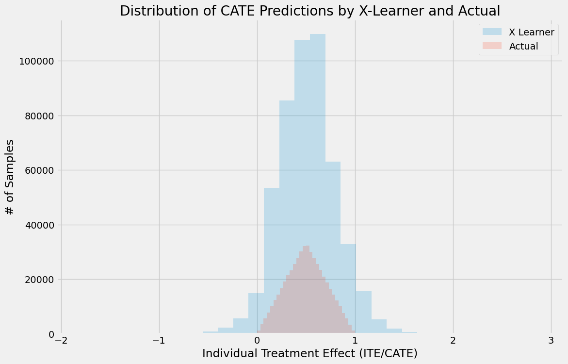
plt.title('Distribution of CATE Predictions by X-Learner and Actual')
plt.xlabel('Individual Treatment Effect (ITE/CATE)')
plt.ylabel('# of Samples')
_=plt.legend()
验证CATE而不使用TMLE
[10]:
df = pd.DataFrame({'y': y_test, 'w': treatment_test, 'tau': tau_test, 'X-Learner': cate_x_test, 'Actual': tau_test})
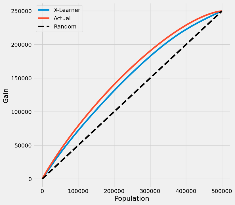
带有真实情况的提升曲线
如果真实治疗效果在模拟中是已知的,模型的提升曲线使用按模型的CATE估计排序的治疗效果的累积和。
在下图中,X-learner的提升曲线显示出接近地面实况最优提升的正向提升。
[11]:
plot(df, outcome_col='y', treatment_col='w', treatment_effect_col='tau')
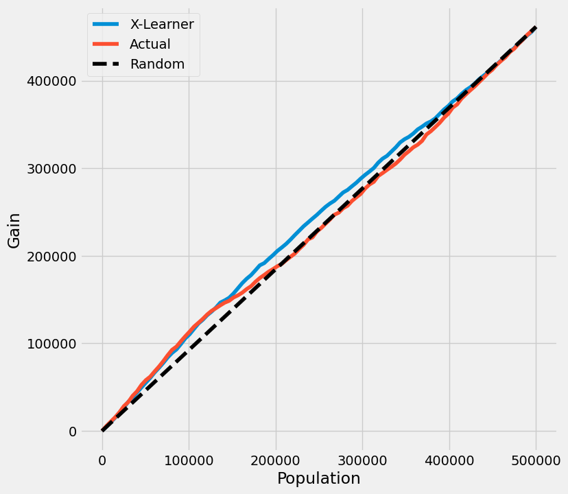
无真实数据的提升曲线
如果真实的治疗效果在实践中未知,模型的提升曲线使用按模型的CATE估计排序的治疗组和对照组结果的累积平均差异。
在下图中,X-learner的提升曲线以及真实情况显示没有提升,这是不正确的。
[12]:
plot(df.drop('tau', axis=1), outcome_col='y', treatment_col='w')
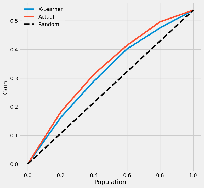
TMLE
以TMLE为基准的提升曲线
通过使用TMLE作为真实情况的代理,X-learner的提升曲线与使用真实情况的原始曲线变得接近。
[13]:
n_fold = 5
kf = KFold(n_splits=n_fold)
[14]:
df = pd.DataFrame({'y': y_test, 'w': treatment_test, 'p': e_test, 'X-Learner': cate_x_test, 'Actual': tau_test})
[15]:
inference_cols = []
for i in range(X_test.shape[1]):
    col = 'col_' + str(i)
    df[col] = X_test[:,i]
    inference_cols.append(col)
[16]:
df.head()
[16]:
| y | w | p | X-Learner | 实际 | col_0 | col_1 | col_2 | col_3 | col_4 | col_5 | col_6 | col_7 | col_8 | col_9 | |
|---|---|---|---|---|---|---|---|---|---|---|---|---|---|---|---|
| 0 | 2.299468 | 0 | 0.875235 | 0.689955 | 0.812923 | 0.801219 | 0.824627 | 0.418361 | 0.576936 | 0.810729 | 0.186007 | 0.883184 | 0.057571 | 0.084963 | 0.782511 |
| 1 | -2.601411 | 1 | 0.715290 | 0.950119 | 0.864145 | 0.885407 | 0.842883 | 0.014536 | 0.974505 | 0.858550 | 0.548230 | 0.164607 | 0.762274 | 0.198254 | 0.647855 |
| 2 | 9.295828 | 1 | 0.895537 | 0.675432 | 0.637853 | 0.406232 | 0.869474 | 0.808828 | 0.525918 | 0.526959 | 0.023063 | 0.903683 | 0.566092 | 0.242138 | 0.219698 |
| 3 | 2.362346 | 0 | 0.230146 | 0.555949 | 0.497591 | 0.914335 | 0.080846 | 0.501873 | 0.912275 | 0.405199 | 0.922577 | 0.054477 | 0.054306 | 0.385622 | 0.244462 |
| 4 | -6.428204 | 1 | 0.772851 | 0.541349 | 0.551009 | 0.700812 | 0.401207 | 0.450781 | 0.988744 | 0.537332 | 0.124579 | 0.700980 | 0.135383 | 0.087629 | 0.198028 |
[17]:
tmle_df = get_tmlegain(df, inference_col=inference_cols, outcome_col='y', treatment_col='w', p_col='p',
                       n_segment=5, cv=kf, calibrate_propensity=True, ci=False)
[LightGBM] [Info] Auto-choosing row-wise multi-threading, the overhead of testing was 0.002342 seconds.
You can set `force_row_wise=true` to remove the overhead.
And if memory is not enough, you can set `force_col_wise=true`.
[LightGBM] [Info] Total Bins 2552
[LightGBM] [Info] Number of data points in the train set: 400000, number of used features: 11
[LightGBM] [Info] Start training from score 1.506199
[LightGBM] [Info] Auto-choosing row-wise multi-threading, the overhead of testing was 0.002307 seconds.
You can set `force_row_wise=true` to remove the overhead.
And if memory is not enough, you can set `force_col_wise=true`.
[LightGBM] [Info] Total Bins 2552
[LightGBM] [Info] Number of data points in the train set: 400000, number of used features: 11
[LightGBM] [Info] Start training from score 1.492271
[LightGBM] [Info] Auto-choosing row-wise multi-threading, the overhead of testing was 0.002273 seconds.
You can set `force_row_wise=true` to remove the overhead.
And if memory is not enough, you can set `force_col_wise=true`.
[LightGBM] [Info] Total Bins 2552
[LightGBM] [Info] Number of data points in the train set: 400000, number of used features: 11
[LightGBM] [Info] Start training from score 1.510604
[LightGBM] [Info] Auto-choosing row-wise multi-threading, the overhead of testing was 0.002306 seconds.
You can set `force_row_wise=true` to remove the overhead.
And if memory is not enough, you can set `force_col_wise=true`.
[LightGBM] [Info] Total Bins 2552
[LightGBM] [Info] Number of data points in the train set: 400000, number of used features: 11
[LightGBM] [Info] Start training from score 1.499669
[LightGBM] [Info] Auto-choosing row-wise multi-threading, the overhead of testing was 0.002286 seconds.
You can set `force_row_wise=true` to remove the overhead.
And if memory is not enough, you can set `force_col_wise=true`.
[LightGBM] [Info] Total Bins 2552
[LightGBM] [Info] Number of data points in the train set: 400000, number of used features: 11
[LightGBM] [Info] Start training from score 1.508310
[LightGBM] [Info] Auto-choosing row-wise multi-threading, the overhead of testing was 0.002342 seconds.
You can set `force_row_wise=true` to remove the overhead.
And if memory is not enough, you can set `force_col_wise=true`.
[LightGBM] [Info] Total Bins 2552
[LightGBM] [Info] Number of data points in the train set: 400000, number of used features: 11
[LightGBM] [Info] Start training from score 1.506199
[LightGBM] [Info] Auto-choosing row-wise multi-threading, the overhead of testing was 0.002269 seconds.
You can set `force_row_wise=true` to remove the overhead.
And if memory is not enough, you can set `force_col_wise=true`.
[LightGBM] [Info] Total Bins 2552
[LightGBM] [Info] Number of data points in the train set: 400000, number of used features: 11
[LightGBM] [Info] Start training from score 1.492271
[LightGBM] [Info] Auto-choosing row-wise multi-threading, the overhead of testing was 0.002360 seconds.
You can set `force_row_wise=true` to remove the overhead.
And if memory is not enough, you can set `force_col_wise=true`.
[LightGBM] [Info] Total Bins 2552
[LightGBM] [Info] Number of data points in the train set: 400000, number of used features: 11
[LightGBM] [Info] Start training from score 1.510604
[LightGBM] [Info] Auto-choosing row-wise multi-threading, the overhead of testing was 0.002696 seconds.
You can set `force_row_wise=true` to remove the overhead.
And if memory is not enough, you can set `force_col_wise=true`.
[LightGBM] [Info] Total Bins 2552
[LightGBM] [Info] Number of data points in the train set: 400000, number of used features: 11
[LightGBM] [Info] Start training from score 1.499669
[LightGBM] [Info] Auto-choosing row-wise multi-threading, the overhead of testing was 0.002270 seconds.
You can set `force_row_wise=true` to remove the overhead.
And if memory is not enough, you can set `force_col_wise=true`.
[LightGBM] [Info] Total Bins 2552
[LightGBM] [Info] Number of data points in the train set: 400000, number of used features: 11
[LightGBM] [Info] Start training from score 1.508310
[LightGBM] [Info] Auto-choosing row-wise multi-threading, the overhead of testing was 0.002288 seconds.
You can set `force_row_wise=true` to remove the overhead.
And if memory is not enough, you can set `force_col_wise=true`.
[LightGBM] [Info] Total Bins 2552
[LightGBM] [Info] Number of data points in the train set: 400000, number of used features: 11
[LightGBM] [Info] Start training from score 1.506199
[LightGBM] [Info] Auto-choosing row-wise multi-threading, the overhead of testing was 0.002326 seconds.
You can set `force_row_wise=true` to remove the overhead.
And if memory is not enough, you can set `force_col_wise=true`.
[LightGBM] [Info] Total Bins 2552
[LightGBM] [Info] Number of data points in the train set: 400000, number of used features: 11
[LightGBM] [Info] Start training from score 1.492271
[LightGBM] [Info] Auto-choosing row-wise multi-threading, the overhead of testing was 0.002311 seconds.
You can set `force_row_wise=true` to remove the overhead.
And if memory is not enough, you can set `force_col_wise=true`.
[LightGBM] [Info] Total Bins 2552
[LightGBM] [Info] Number of data points in the train set: 400000, number of used features: 11
[LightGBM] [Info] Start training from score 1.510604
[LightGBM] [Info] Auto-choosing row-wise multi-threading, the overhead of testing was 0.002322 seconds.
You can set `force_row_wise=true` to remove the overhead.
And if memory is not enough, you can set `force_col_wise=true`.
[LightGBM] [Info] Total Bins 2552
[LightGBM] [Info] Number of data points in the train set: 400000, number of used features: 11
[LightGBM] [Info] Start training from score 1.499669
[LightGBM] [Info] Auto-choosing row-wise multi-threading, the overhead of testing was 0.002287 seconds.
You can set `force_row_wise=true` to remove the overhead.
And if memory is not enough, you can set `force_col_wise=true`.
[LightGBM] [Info] Total Bins 2552
[LightGBM] [Info] Number of data points in the train set: 400000, number of used features: 11
[LightGBM] [Info] Start training from score 1.508310
[18]:
tmle_df
[18]:
| X-Learner | 实际值 | |
|---|---|---|
| 0.0 | 0.000000 | 0.000000 |
| 0.2 | 0.162729 | 0.181960 |
| 0.4 | 0.289292 | 0.312707 |
| 0.6 | 0.401203 | 0.413857 |
| 0.8 | 0.474771 | 0.496008 |
| 1.0 | 0.536501 | 0.536501 |
无置信区间的提升曲线
在这里我们可以直接使用plot_tmle()函数来生成结果并绘制提升曲线
[19]:
plot_tmlegain(df, inference_col=inference_cols, outcome_col='y', treatment_col='w', p_col='p',
              n_segment=5, cv=kf, calibrate_propensity=True, ci=False)

我们还提供了直接使用plot()的API调用,通过输入kind='gain'和tmle=True
[20]:
plot(df, kind='gain', tmle=True, inference_col=inference_cols, outcome_col='y', treatment_col='w', p_col='p',
     n_segment=5, cv=kf, calibrate_propensity=True, ci=False)
AUUC 分数
[21]:
auuc_score(df, tmle=True, inference_col=inference_cols, outcome_col='y', treatment_col='w', p_col='p',
           n_segment=5, cv=kf, calibrate_propensity=True, ci=False)
[21]:
X-Learner    0.310749
Actual       0.323505
dtype: float64
带有置信区间的提升曲线
[22]:
tmle_df = get_tmlegain(df, inference_col=inference_cols, outcome_col='y', treatment_col='w', p_col='p',
                       n_segment=5, cv=kf, calibrate_propensity=True, ci=True)
[23]:
tmle_df
[23]:
| X-Learner | 实际值 | X-Learner 下限 | 实际值 下限 | X-Learner 上限 | 实际值 上限 | |
|---|---|---|---|---|---|---|
| 0.0 | 0.000000 | 0.000000 | 0.000000 | 0.000000 | 0.000000 | 0.000000 |
| 0.2 | 0.162729 | 0.181960 | 0.144712 | 0.162806 | 0.180746 | 0.201114 |
| 0.4 | 0.289292 | 0.312707 | 0.253433 | 0.275556 | 0.325151 | 0.349859 |
| 0.6 | 0.401203 | 0.413857 | 0.349491 | 0.362746 | 0.452916 | 0.464968 |
| 0.8 | 0.474771 | 0.496008 | 0.407328 | 0.429929 | 0.542213 | 0.562086 |
| 1.0 | 0.536501 | 0.536501 | 0.498278 | 0.498278 | 0.574724 | 0.574724 |
[24]:
plot_tmlegain(df, inference_col=inference_cols, outcome_col='y', treatment_col='w', p_col='p',
              n_segment=5, cv=kf, calibrate_propensity=True, ci=True)
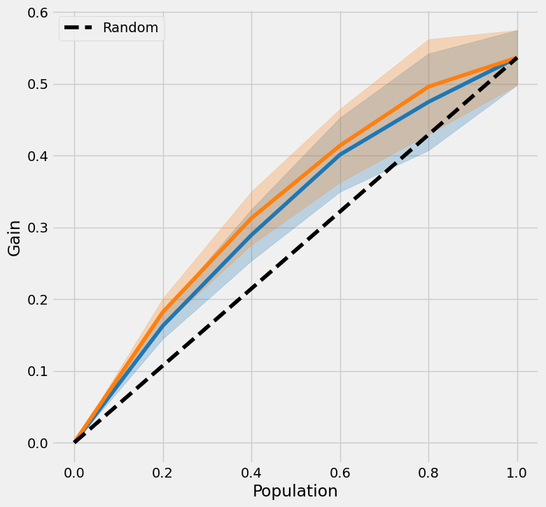
[25]:
plot(df, kind='gain', tmle=True, inference_col=inference_cols, outcome_col='y', treatment_col='w', p_col='p',
     n_segment=5, cv=kf, calibrate_propensity=True, ci=True)

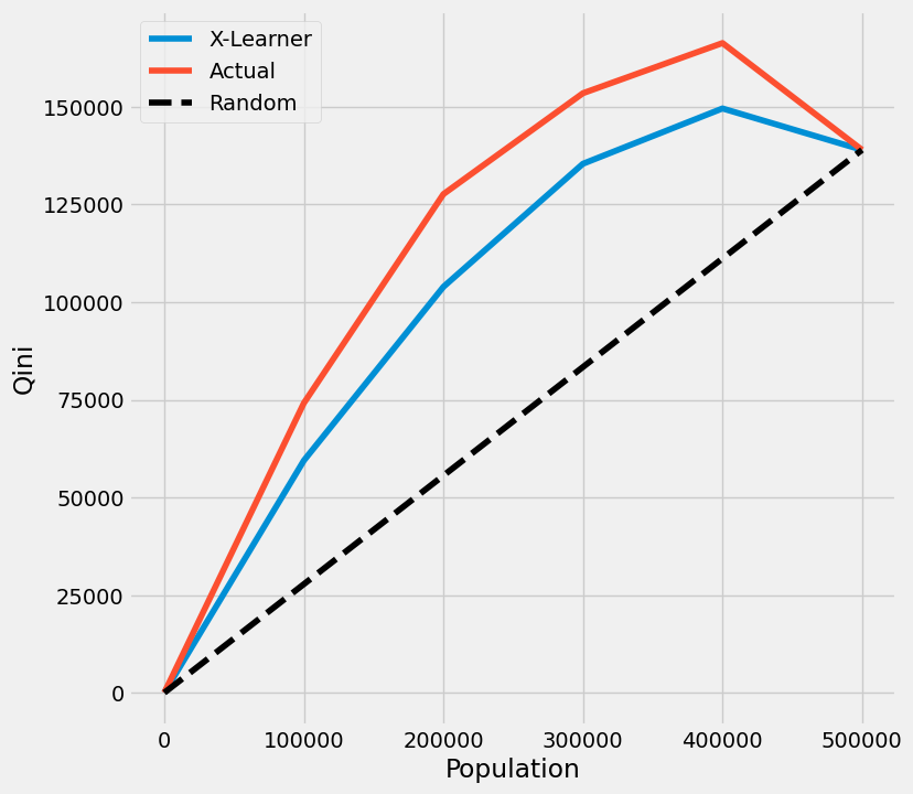
以TMLE为基准的Qini曲线
无置信区间的基尼曲线
[26]:
qini = get_tmleqini(df, inference_col=inference_cols, outcome_col='y', treatment_col='w', p_col='p',
                    n_segment=5, cv=kf, calibrate_propensity=True, ci=False)
[27]:
qini
[27]:
| X-Learner | 实际值 | |
|---|---|---|
| 0.0 | 0.000000 | 0.000000 |
| 100000.0 | 59451.339999 | 74162.340931 |
| 200000.0 | 103923.696240 | 127661.597180 |
| 300000.0 | 135436.896364 | 153502.216545 |
| 400000.0 | 149594.578171 | 166344.875062 |
| 500000.0 | 138989.103266 | 138989.103266 |
[28]:
plot_tmleqini(df, inference_col=inference_cols, outcome_col='y', treatment_col='w', p_col='p',
              n_segment=5, cv=kf, calibrate_propensity=True, ci=False)

我们还提供了直接使用plot()的API调用,通过输入kind='qini'和tmle=True
[29]:
plot(df, kind='qini', tmle=True, inference_col=inference_cols, outcome_col='y', treatment_col='w', p_col='p',
     n_segment=5, cv=kf, calibrate_propensity=True, ci=False)
七牛评分
[30]:
qini_score(df, tmle=True, inference_col=inference_cols, outcome_col='y', treatment_col='w', p_col='p',
           n_segment=5, cv=kf, calibrate_propensity=True, ci=False)
[30]:
X-Learner    28404.717374
Actual       40615.470531
Random           0.000000
dtype: float64
带有置信区间的基尼曲线
[31]:
qini = get_tmleqini(df, inference_col=inference_cols, outcome_col='y', treatment_col='w', p_col='p',
                    n_segment=5, cv=kf, calibrate_propensity=True, ci=True)
[32]:
qini
[32]:
| X-Learner | 实际值 | X-Learner 下限 | 实际值 下限 | X-Learner 上限 | 实际值 上限 | |
|---|---|---|---|---|---|---|
| 0.0 | 0.000000 | 0.000000 | 0.000000 | 0.000000 | 0.000000 | 0.000000 |
| 100000.0 | 59451.339999 | 74162.340931 | 52869.065243 | 66355.766067 | 66033.614756 | 81968.915795 |
| 200000.0 | 103923.696240 | 127661.597180 | 91071.983173 | 112490.548288 | 116775.409307 | 142832.646073 |
| 300000.0 | 135436.896364 | 153502.216545 | 118121.046182 | 134765.053280 | 152752.746546 | 172239.379810 |
| 400000.0 | 149594.578171 | 166344.875062 | 129251.502323 | 145267.815499 | 169937.654019 | 187421.934626 |
| 500000.0 | 138989.103266 | 138989.103266 | 138989.103266 | 138989.103266 | 138989.103266 | 138989.103266 |
[33]:
plot_tmleqini(df, inference_col=inference_cols, outcome_col='y', treatment_col='w', p_col='p',
              n_segment=5, cv=kf, calibrate_propensity=True, ci=True)
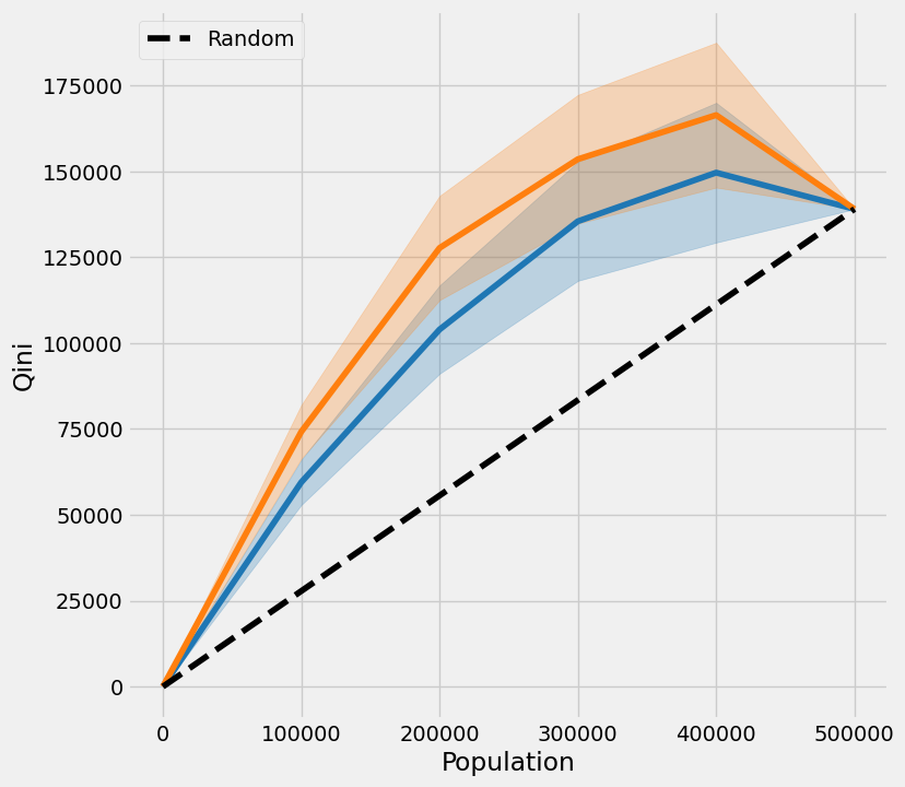
[34]:
plot(df, kind='qini', tmle=True, inference_col=inference_cols, outcome_col='y', treatment_col='w', p_col='p',
     n_segment=5, cv=kf, calibrate_propensity=True, ci=True)
