D4PG¶

概述¶

D4PG，在论文分布式分布确定性策略梯度中提出，是一种基于演员-评论家的无模型策略梯度算法，它扩展了DDPG。与DDPG相比，改进包括使用N步回报、优先经验回放和分布价值函数。此外，训练通过多个分布式工作器并行进行，所有工作器都写入同一个回放表。作者发现，这些简单的修改有助于算法的整体性能，其中N步回报带来了最大的性能提升，而优先缓冲的重要性相对较小。

快速事实¶

D4PG仅用于具有连续动作空间的环境。（例如MuJoCo）
D4PG 是一种 离策略 算法。
D4PG 使用了一个分布式的评论家。
D4PG 是一种无模型和演员-评论家强化学习算法，分别优化演员网络和评论家网络。
通常，D4PG使用Ornstein-Uhlenbeck过程或高斯过程（在我们的实现中默认）进行探索。

关键方程或关键图表¶

D4PG算法维护一个分布评论家\(Z_\pi(s, a)\)，它将预期的Q值估计为一个随机变量，使得\(Q(s, a)=\mathbb{E}Z_\pi(s, a)\)。\(Z\)通常是Q的51个支撑点的分类分布。

因此，分布贝尔曼算子可以定义为：

\[\begin{aligned} (\mathcal{T}_{\pi} Z)(s, a)=r(s, a)+\gamma\mathbb{E}[Z(s',\pi(s'))|(s, a)] \end{aligned}\]

该操作符的分布变体接受从状态-动作对映射到分布的函数，并返回相同形式的函数。用于学习评论者分布参数的损失定义为\(L(\pi) = \mathbb{E}[d(\mathcal{T}_{\pi_{\theta'}}, Z_{w'}(s, a), Z_{w}(s, a)]\) 对于某些度量\(d\)，它测量两个分布之间的距离。

最后，通过考虑动作值分布的期望来完成演员更新：

\[\begin{split}\begin{aligned} \nabla_\theta J(\theta) &\approx \mathbb{E}_{\rho^\pi} [\nabla_a Q_w(s, a) \nabla_\theta \pi_{\theta}(s) \rvert_{a=\pi\theta(s)}] \\ &= \mathbb{E}_{\rho^\pi} [\mathbb{E}[\nabla_a Z_w(s, a)] \nabla_\theta \pi_{\theta}(s) \rvert_{a=\pi\theta(s)}] \end{aligned}\end{split}\]

在计算TD误差时，D4PG计算TD目标中的N步以包含更多未来步骤的奖励：

\[r(s_0, a_0) + \mathbb{E}[\sum_{n=1}^{N-1} \gamma^n r(s_n, a_n) + \gamma^N Q(s_N, \mu_\theta(s_N)) \vert s_0, a_0 ]\]

D4PG 从优先回放缓冲区中以非均匀概率 \(p_i\) 进行采样。这需要使用重要性采样，通过将评论家更新加权一个因子 \(R_{p_i}^{-1}\) 来实现。

注意

D4PG 利用多个并行独立演员，收集经验并将数据输入到同一个回放缓冲区。然而，我们的实现仅使用单个演员。

伪代码¶

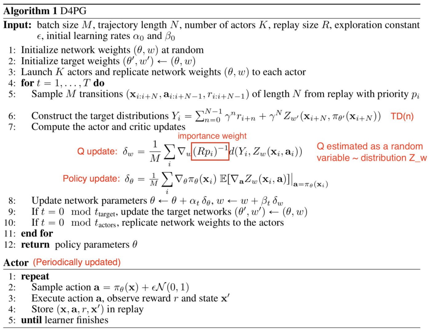
../_images/D4PG_algo.png — 来源: https://lilianweng.github.io/posts/2018-04-08-policy-gradient/#d4pg¶

实现¶

默认配置定义如下：

class ding.policy.d4pg.D4PGPolicy(cfg: EasyDict, model: Module | None = None, enable_field: List[str] | None = None)[来源]

Overview:

D4PG算法的策略类。D4PG是DDPG的一个变体，它使用分布式的评论家。分布式评论家通过使用分位数回归来实现。论文链接：https://arxiv.org/abs/1804.08617。

Property:

学习模式, 收集模式, 评估模式

Config:

ID	符号	类型	默认值	描述	其他（形状）
1	`type`	字符串	d4pg	RL policy register name, refer to registry `POLICY_REGISTRY`	this arg is optional, a placeholder
2	`cuda`	布尔	真	Whether to use cuda for network
3	`random_` `collect_size`	整数	25000	Number of randomly collected training samples in replay buffer when training starts.	Default to 25000 for DDPG/TD3, 10000 for sac.
5	`learn.learning` `_rate_actor`	浮点数	1e-3	Learning rate for actor network(aka. policy).
6	`learn.learning` `_rate_critic`	浮点数	1e-3	Learning rates for critic network (aka. Q-network).
7	`learn.actor_` `update_freq`	整数	1	When critic network updates once, how many times will actor network update.	Default 1
8	`learn.noise`	布尔	假	Whether to add noise on target network’s action.	Default False for D4PG. Target Policy Smoo- thing Regularization in TD3 paper.
9	`learn.-` `ignore_done`	布尔	假	Determine whether to ignore done flag.	Use ignore_done only in halfcheetah env.
10	`learn.-` `target_theta`	浮点数	0.005	Used for soft update of the target network.	aka. Interpolation factor in polyak aver aging for target networks.
11	`collect.-` `noise_sigma`	浮点数	0.1	Used for add noise during co- llection, through controlling the sigma of distribution	Sample noise from dis tribution, Gaussian process.
12	`model.v_min`	浮点数	-10	Value of the smallest atom in the support set.
13	`model.v_max`	浮点数	10	Value of the largest atom in the support set.
14	`model.n_atom`	整数	51	Number of atoms in the support set of the value distribution.
15	`nstep`	整数	3, [1, 5]	N-step reward discount sum for target q_value estimation
16	`priority`	布尔	真	Whether use priority(PER)	priority sample, update priority

模型¶

这里我们提供了QACDIST模型作为D4PG的默认模型的示例。

class ding.model.template.qac_dist.QACDIST(obs_shape: int | SequenceType, action_shape: int | SequenceType, action_space: str = 'regression', critic_head_type: str = 'categorical', actor_head_hidden_size: int = 64, actor_head_layer_num: int = 1, critic_head_hidden_size: int = 64, critic_head_layer_num: int = 1, activation: Module | None = ReLU(), norm_type: str | None = None, v_min: float | None = -10, v_max: float | None = 10, n_atom: int | None = 51)[源代码]

Overview:: 具有分布Q值的QAC模型。
Interfaces:: __init__, forward, compute_actor, compute_critic

compute_actor(inputs: Tensor) → Dict[source]

Overview:

使用编码的嵌入张量来预测输出。使用'compute_actor'模式执行参数更新使用编码的嵌入张量来预测输出。

Arguments:

inputs (torch.Tensor):
编码后的嵌入张量，由给定的hidden_size决定，即(B, N=hidden_size)。 hidden_size = actor_head_hidden_size
模式 (str): 前向模式的名称。

Returns:

输出 (Dict): 前向传递编码器和头部的输出。

ReturnsKeys (either):

动作 (torch.Tensor): 与 action_shape 大小相同的连续动作张量。
logit (torch.Tensor):
Logit 张量编码 mu 和 sigma，两者的大小与输入 x 相同。

Shapes:

输入 (torch.Tensor): \((B, N0)\), B 是批量大小，N0 对应于 hidden_size
动作 (torch.Tensor): \((B, N0)\)
logit (list): 2个元素，mu和sigma，每个的形状为\((B, N0)\)。
q_value (torch.FloatTensor): \((B, )\), B 是批量大小。

Examples:

>>> # Regression mode
>>> model = QACDIST(64, 64, 'regression')
>>> inputs = torch.randn(4, 64)
>>> actor_outputs = model(inputs,'compute_actor')
>>> assert actor_outputs['action'].shape == torch.Size([4, 64])
>>> # Reparameterization Mode
>>> model = QACDIST(64, 64, 'reparameterization')
>>> inputs = torch.randn(4, 64)
>>> actor_outputs = model(inputs,'compute_actor')
>>> actor_outputs['logit'][0].shape # mu
>>> torch.Size([4, 64])
>>> actor_outputs['logit'][1].shape # sigma
>>> torch.Size([4, 64])

compute_critic(inputs: Dict) → Dict[来源]

Overview:

使用'compute_critic'模式执行参数更新使用编码的嵌入张量来预测输出。

Arguments:

obs, action 编码的张量。
模式 (str): 前向模式的名称。

Returns:

输出 (Dict): Q值输出和分布。

ReturnKeys:

q_value (torch.Tensor): Q值张量，大小与批量大小相同。
分布 (torch.Tensor): Q值分布张量。

Shapes:

obs (torch.Tensor): \((B, N1)\), 其中 B 是批量大小，N1 是 obs_shape
动作 (torch.Tensor): \((B, N2)\), 其中 B 是批量大小，N2 是``action_shape``
q_value (torch.FloatTensor): \((B, N2)\), 其中 B 是批量大小，N2 是 action_shape
分布 (torch.FloatTensor): \((B, 1, N3)\), 其中 B 是批量大小，N3 是 num_atom

Examples:

>>> # Categorical mode
>>> inputs = {'obs': torch.randn(4,N), 'action': torch.randn(4,1)}
>>> model = QACDIST(obs_shape=(N, ),action_shape=1,action_space='regression',             ...                 critic_head_type='categorical', n_atoms=51)
>>> q_value = model(inputs, mode='compute_critic') # q value
>>> assert q_value['q_value'].shape == torch.Size([4, 1])
>>> assert q_value['distribution'].shape == torch.Size([4, 1, 51])

forward(inputs: Tensor | Dict, mode: str) → Dict[来源]

Overview:

使用观察和动作张量来预测输出。参数更新使用QACDIST的MLPs前向设置。

Arguments:

Forward with 'compute_actor':

inputs (torch.Tensor):
编码的嵌入张量，由给定的hidden_size决定，即(B, N=hidden_size)。是actor_head_hidden_size还是critic_head_hidden_size取决于mode。

Forward with 'compute_critic', inputs (Dict) Necessary Keys:

obs, action 编码的张量。

模式 (str): 前向模式的名称。

Returns:

输出 (Dict): 网络前向的输出。
Forward with 'compute_actor', Necessary Keys (either):
动作 (torch.Tensor): 与输入 x 大小相同的动作张量。

logit (torch.Tensor):
Logit 张量编码 mu 和 sigma，两者的大小与输入 x 相同。
Forward with 'compute_critic', Necessary Keys:
q_value (torch.Tensor): Q值张量，大小与批量大小相同。

分布 (torch.Tensor): Q值分布张量。

Actor Shapes:

输入 (torch.Tensor): \((B, N0)\), B 是批量大小，N0 对应于 hidden_size
动作 (torch.Tensor): \((B, N0)\)
q_value (torch.FloatTensor): \((B, )\), 其中 B 是批量大小。

Critic Shapes:

obs (torch.Tensor): \((B, N1)\), 其中 B 是批量大小，N1 是 obs_shape
动作 (torch.Tensor): \((B, N2)\), 其中 B 是批量大小，N2 是``action_shape``
q_value (torch.FloatTensor): \((B, N2)\), 其中 B 是批量大小，N2 是 action_shape
分布 (torch.FloatTensor): \((B, 1, N3)\), 其中 B 是批量大小，N3 是 num_atom

Actor Examples:

>>> # Regression mode
>>> model = QACDIST(64, 64, 'regression')
>>> inputs = torch.randn(4, 64)
>>> actor_outputs = model(inputs,'compute_actor')
>>> assert actor_outputs['action'].shape == torch.Size([4, 64])
>>> # Reparameterization Mode
>>> model = QACDIST(64, 64, 'reparameterization')
>>> inputs = torch.randn(4, 64)
>>> actor_outputs = model(inputs,'compute_actor')
>>> actor_outputs['logit'][0].shape # mu
>>> torch.Size([4, 64])
>>> actor_outputs['logit'][1].shape # sigma
>>> torch.Size([4, 64])

Critic Examples:

>>> # Categorical mode
>>> inputs = {'obs': torch.randn(4,N), 'action': torch.randn(4,1)}
>>> model = QACDIST(obs_shape=(N, ),action_shape=1,action_space='regression',             ...                 critic_head_type='categorical', n_atoms=51)
>>> q_value = model(inputs, mode='compute_critic') # q value
>>> assert q_value['q_value'].shape == torch.Size([4, 1])
>>> assert q_value['distribution'].shape == torch.Size([4, 1, 51])

基准测试¶

环境

最佳平均奖励

评估结果

配置链接

比较

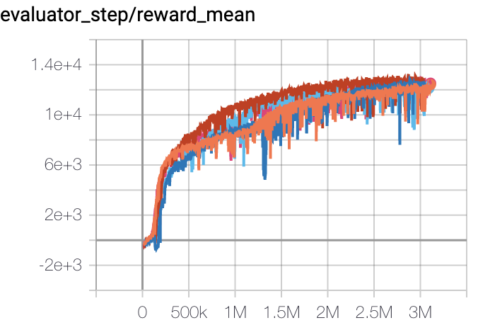
猎豹

(Halfcheetah-v3)

13000

config_link_ha

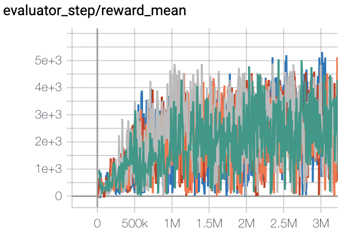
Walker2d

(Walker2d-v2)

5300

config_link_w

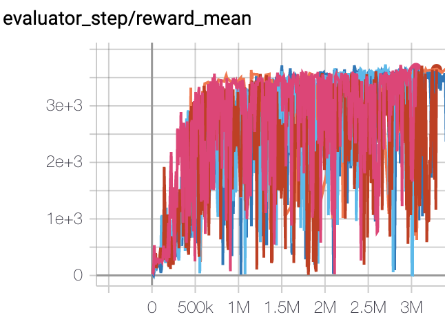
霍珀

(Hopper-v2)

3500

config_link_ho

其他公共实现¶

D4PG Pytorch

参考文献¶

Gabriel Barth-Maron, Matthew W. Hoffman, David Budden, Will Dabney, Dan Horgan, Dhruva TB, Alistair Muldal, Nicolas Heess, Timothy Lillicrap: “分布式分布确定性策略梯度”, 2018; [https://arxiv.org/abs/1804.08617v1 arXiv:1804.08617v1].