IMPALA
概述
IMPALA,即重要性加权演员学习者架构,是一种离策略的演员-评论家框架,它将数据收集与学习分离,并使用离策略校正V-trace从经验轨迹中优化策略。该方法首次在IMPALA: Scalable Distributed Deep-RL with Importance Weighted Actor-Learner Architectures中介绍。
快速事实
IMPALA 是一种无模型和离策略的强化学习算法。
IMPALA 可以支持离散动作空间和连续动作空间。
IMPALA 是一种带有价值网络的演员-评论家强化学习算法,它分别优化演员网络和评论家(价值)网络。
IMPALA 可以利用旧的离策略数据,通过相应的离策略校正来稳定学习。
IMPALA 将数据收集与学习解耦。IMPALA 中的收集器不会计算价值或优势。
IMPALA 是一种分布式 RL 架构,采用经典的演员-学习者范式。
关键公式
IMPALA中使用的损失与PPO、A2C和其他价值函数演员-评论家模型中的损失类似。它们都来自于policy_loss、value_loss和entropy_loss,并根据一些精心选择的权重进行计算,即:
提示
符号和约定:
\(\pi_{\phi}\): 当前由\(\phi\)参数化的训练策略。
\(V_\theta\): 由\(\theta\)参数化的价值函数。
\(\mu\): 旧策略,用于在回放缓冲区中生成轨迹。
在训练时间 \(t\),给定转换 \((x_t, a_t, x_{t+1}, r_t)\),价值函数 \(V_\theta\) 通过当前价值与V-trace目标价值之间的\(L_2\)损失进行学习。时间s处的n步V-trace目标 定义如下:
其中 \(\delta_t V \stackrel{def}{=} \rho_t (r_t + \gamma V(x_{t+1}) - V(x_t))\) 是 \(V\) 的时间差分, \(\rho_t \stackrel{def}{=} \min\big(\bar{\rho}, \frac{\pi(a_t \vert x_t)}{\mu(a_t \vert x_t)}\big)\), 以及 \(c_i \stackrel{def}{=}\min\big(\bar{c}, \frac{\pi(a_i \vert s_i)}{\mu(a_i \vert s_i)}\big)\)
\(\rho_t\) 和 \(c_i\) 是 truncated importance sampling (IS) weights,
其中 \(\bar{\rho}\) 和 \(\bar{c}\) 是两个截断常数,且 \(\bar{\rho} \geq \bar{c}\)。
乘积 \(c_s, \dots, c_{t-1}\) 衡量了在时间 \(t\) 观察到的时间差分 \(\delta_t V\) 对先前时间 \(s\) 的值函数更新的影响。在策略内的情况下,我们有 \(\rho_t=1\) 和 \(c_i=1\)(假设 \(\bar{c} \geq 1)\),因此 V-trace 目标变为策略内的 n 步贝尔曼目标。
注意
\(\bar{\rho}\) 影响我们收敛到的价值函数的不动点,而 \(\bar{c}\) 影响收敛速度。
当 \(\bar{\rho} =\infty\)(未截断)时,v-trace 值函数将收敛到目标策略的值函数 \(V_\pi\);
当\(\bar{\rho}\)接近0时,我们评估行为策略\(V_\mu\)的价值函数;当处于中间值时,我们评估介于\(\pi\)和\(\mu\)之间的策略。
因此,损失函数是
其中 \(H(\pi_{\phi})\),策略 \(\phi\) 的熵,是鼓励探索的奖励。
价值函数参数更新方向为:
策略参数 \(\phi\) 通过策略梯度更新,
其中 \(r_s + \gamma v_{s+1}\) 是 v-trace 优势,它是估计的 Q 值减去一个依赖于状态的基线 \(V_\theta(x_s)\)。
关键图表
下图描述了IMPALA原始论文中的分布式架构。然而,我们的实现与原始论文中的略有不同。
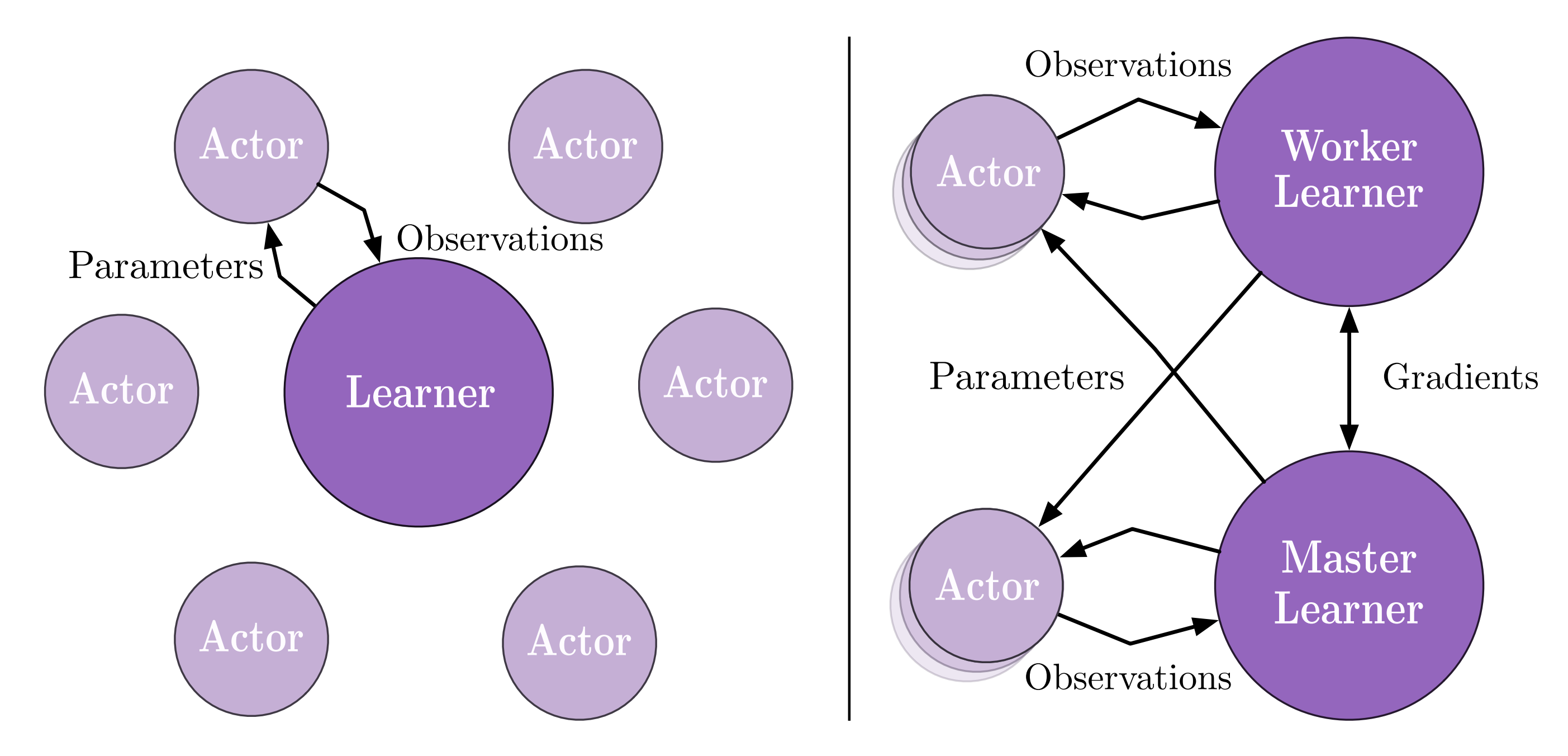
对于单个学习者,他们使用多个演员/收集器来生成训练数据。而在我们的设置中,我们使用一个具有多个环境的收集器来增加数据的多样性。
对于多个学习者,在原始论文中,不同的学习者将拥有不同的演员。换句话说,他们将拥有不同的ReplayBuffer。而在我们的设置中,所有的学习者将共享同一个ReplayBuffer,并在每次迭代后同步。
实现
配置
默认配置定义如下:
- class ding.policy.impala.IMPALAPolicy(cfg: EasyDict, model: Module | None = None, enable_field: List[str] | None = None)[source]
- Overview:
IMPALA算法的策略类。论文链接:https://arxiv.org/abs/1802.01561。
- Config:
ID
符号
类型
默认值
描述
其他(形状)
1
type字符串
impala
RL policy register name, refer toregistryPOLICY_REGISTRYthis arg is optional,a placeholder2
cuda布尔
假
Whether to use cuda for networkthis arg can be diff-erent from modes3
on_policy布尔
假
Whether the RL algorithm is on-policyor off-policypriority布尔
假
Whether use priority(PER)priority sample,update priority5
priority_IS_weight布尔
假
Whether use Importance Sampling WeightIf True, prioritymust be True6
unroll_len整数
32
trajectory length to calculate v-tracetarget7
learn.updateper_collect整数
4
How many updates(iterations) to trainafter collector’s one collection. Onlyvalid in serial trainingthis args can be varyfrom envs. Bigger valmeans more off-policy
IMPALA 使用的网络接口定义如下:
- class ding.model.template.vac.VAC(obs_shape: int | SequenceType, action_shape: int | SequenceType | EasyDict, action_space: str = 'discrete', share_encoder: bool = True, encoder_hidden_size_list: SequenceType = [128, 128, 64], actor_head_hidden_size: int = 64, actor_head_layer_num: int = 1, critic_head_hidden_size: int = 64, critic_head_layer_num: int = 1, activation: Module | None = ReLU(), norm_type: str | None = None, sigma_type: str | None = 'independent', fixed_sigma_value: int | None = 0.3, bound_type: str | None = None, encoder: Module | None = None, impala_cnn_encoder: bool = False)[source]
- Overview:
与(状态)值演员-评论家(VAC)相关的算法的神经网络和计算图,例如A2C/PPO/IMPALA。该模型现在支持离散、连续和混合动作空间。VAC由四部分组成:
actor_encoder、critic_encoder、actor_head和critic_head。编码器用于从各种观察中提取特征。头部用于预测相应的值或动作逻辑。在高维观察空间(如2D图像)中,我们通常为actor_encoder和critic_encoder使用共享编码器。在低维观察空间(如1D向量)中,我们通常使用不同的编码器。- Interfaces:
__init__,forward,compute_actor,compute_critic,compute_actor_critic.
- forward(x: Tensor, mode: str) Dict[source]
- Overview:
VAC前向计算图,输入观测张量以预测状态值或动作逻辑。不同的
mode将使用不同的网络模块进行前向传播,以获得不同的输出并节省计算。- Arguments:
x (
torch.Tensor): 输入的观测张量数据。模式 (
str): 前向模式,所有模式都在这个类的开头定义。- Returns:
输出 (
Dict): VAC前向计算图的输出字典,其键值因不同的mode而异。- Examples (Actor):
- Examples (Critic):
- Examples (Actor-Critic):
数据处理
通常,我们希望以批处理的方式计算所有内容以提高效率。特别是在计算vtrace时,我们需要所有训练样本(训练数据序列)具有相同的长度。这是在policy._get_train_sample中完成的。一旦我们在收集器中执行此函数,样本的长度将等于配置中的unroll_len。有关详细信息,请参阅ding.rl_utils.adder的文档。
def _get_train_sample(self, data: List[Dict[str, Any]]) -> List[Dict[str, Any]]:
    return get_train_sample(data, self._unroll_len)

def get_train_sample(cls, data: List[Dict[str, Any]], unroll_len: int, last_fn_type: str = 'last') -> List[Dict[str, Any]]:
    """
    Overview:
        Process raw traj data by updating keys ['next_obs', 'reward', 'done'] in data's dict element.
        If ``unroll_len`` equals to 1, which means no process is needed, can directly return ``data``.
        Otherwise, ``data`` will be split according to ``self._unroll_len``, process residual part according to
        ``last_fn_type`` and call ``lists_to_dicts`` to form sampled training data.
    Arguments:
        - data (:obj:`List[Dict[str, Any]]`): transitions list, each element is a transition dict
    Returns:
        - data (:obj:`List[Dict[str, Any]]`): transitions list processed after unrolling
    """
    if unroll_len == 1:
        return data
    else:
        # cut data into pieces whose length is unroll_len
        split_data, residual = list_split(data, step=self._unroll_len)

        def null_padding():
            template = copy.deepcopy(residual[0])
            template['done'] = True
            template['reward'] = torch.zeros_like(template['reward'])
            if 'value_gamma' in template:
                template['value_gamma'] = 0.
            null_data = [cls._get_null_transition(template) for _ in range(miss_num)]
            return null_data

        if residual is not None:
            miss_num = unroll_len - len(residual)
            if last_fn_type == 'drop':
                # drop the residual part
                pass
            elif last_fn_type == 'last':
                if len(split_data) > 0:
                    # copy last datas from split_data's last element, and insert in front of residual
                    last_data = copy.deepcopy(split_data[-1][-miss_num:])
                    split_data.append(last_data + residual)
                else:
                    # get null transitions using ``null_padding``, and insert behind residual
                    null_data = null_padding()
                    split_data.append(residual + null_data)
            elif last_fn_type == 'null_padding':
                # same to the case of 'last' type and split_data is empty
                null_data = null_padding()
                split_data.append(residual + null_data)
        # collate unroll_len dicts according to keys
        if len(split_data) > 0:
            split_data = [lists_to_dicts(d, recursive=True) for d in split_data]
        return split_data
注意
在get_train_sample中,我们介绍了三种将轨迹数据切割成相同长度片段的方法(长度等于unroll_len)。
1. 第一个是 drop,这意味着在将轨迹数据分割成小块后,我们简单地丢弃那些长度小于 unroll_len 的数据。这种方法有些天真,通常不是一个好的选择。因为在强化学习中,一个情节中的最后几个数据通常非常重要,我们不能就这样丢弃它们。
2. 第二种方法是 last,这意味着如果轨迹的总长度小于 unroll_len,我们将使用零填充。否则,我们将使用前一段的数据来填充剩余的部分。此方法设置为默认并推荐使用。
最后一种方法
null_padding只是零填充,这种方法效率不高,因为很多数据会是null。
优化
现在,我们介绍vtrace-value的计算。
首先,我们使用以下函数来计算importance_weights。
def compute_importance_weights(target_output, behaviour_output, action, requires_grad=False):
    """
    Shapes:
        - target_output (:obj:`torch.FloatTensor`): :math:`(T, B, N)`, where T is timestep, B is batch size and\
            N is action dim
        - behaviour_output (:obj:`torch.FloatTensor`): :math:`(T, B, N)`
        - action (:obj:`torch.LongTensor`): :math:`(T, B)`
        - rhos (:obj:`torch.FloatTensor`): :math:`(T, B)`
    """

    grad_context = torch.enable_grad() if requires_grad else torch.no_grad()
    assert isinstance(action, torch.Tensor)
    device = action.device

    with grad_context:
        dist_target = torch.distributions.Categorical(logits=target_output)
        dist_behaviour = torch.distributions.Categorical(logits=behaviour_output)
        rhos = dist_target.log_prob(action) - dist_behaviour.log_prob(action)
        rhos = torch.exp(rhos)
        return rhos
之后,我们根据常数 \(\rho\) 和 \(c\) 裁剪重要性权重,得到 clipped_rhos 和 clipped_cs。 然后我们可以根据以下函数计算 vtrace 值。注意,这里的 bootstrap_values 只是 vtrace 定义中的值函数 \(V(x_s)\)。
def vtrace_nstep_return(clipped_rhos, clipped_cs, reward, bootstrap_values, gamma=0.99, lambda_=0.95):
    """
    Shapes:
        - clipped_rhos (:obj:`torch.FloatTensor`): :math:`(T, B)`, where T is timestep, B is batch size
        - clipped_cs (:obj:`torch.FloatTensor`): :math:`(T, B)`
        - reward: (:obj:`torch.FloatTensor`): :math:`(T, B)`
        - bootstrap_values (:obj:`torch.FloatTensor`): :math:`(T+1, B)`
        - vtrace_return (:obj:`torch.FloatTensor`):  :math:`(T, B)`
    """
    deltas = clipped_rhos * (reward + gamma * bootstrap_values[1:] - bootstrap_values[:-1])
    factor = gamma * lambda_
    result = bootstrap_values[:-1].clone()
    vtrace_item = 0.
    for t in reversed(range(reward.size()[0])):
        vtrace_item = deltas[t] + factor * clipped_cs[t] * vtrace_item
        result[t] += vtrace_item
    return result
注意
1. 此部分中的Bootstrap_values需要具有大小(T+1,B),其中T是时间步长,B是批量大小。原因是
我们需要一个具有相同长度vtrace值的训练数据序列(此长度就是配置中的unroll_len)。
并且为了计算序列中的最后一个vtrace值,我们至少还需要一个目标值。这是
通过使用训练数据序列中最后一个转换的下一个观察值来完成的。
2. 这里我们引入了一个参数 lambda_,遵循AlphaStar中的实现。该参数介于0和1之间,可以对vtrace的离策略校正进行微妙的控制。通常,我们会选择这个参数接近1。
一旦我们获得了vtrace值,或者vtrace_nstep_return,损失函数的计算就变得直接了。整个过程如下。
def vtrace_advantage(clipped_pg_rhos, reward, return_, bootstrap_values, gamma):
    """
    Shapes:
        - clipped_pg_rhos (:obj:`torch.FloatTensor`): :math:`(T, B)`, where T is timestep, B is batch size
        - reward: (:obj:`torch.FloatTensor`): :math:`(T, B)`
        - return_ (:obj:`torch.FloatTensor`):  :math:`(T, B)`
        - bootstrap_values (:obj:`torch.FloatTensor`): :math:`(T, B)`
        - vtrace_advantage (:obj:`torch.FloatTensor`):  :math:`(T, B)`
    """
    return clipped_pg_rhos * (reward + gamma * return_ - bootstrap_values)

def vtrace_error(
        data: namedtuple,
        gamma: float = 0.99,
        lambda_: float = 0.95,
        rho_clip_ratio: float = 1.0,
        c_clip_ratio: float = 1.0,
        rho_pg_clip_ratio: float = 1.0):
    """
    Shapes:
        - target_output (:obj:`torch.FloatTensor`): :math:`(T, B, N)`, where T is timestep, B is batch size and\
            N is action dim
        - behaviour_output (:obj:`torch.FloatTensor`): :math:`(T, B, N)`
        - action (:obj:`torch.LongTensor`): :math:`(T, B)`
        - value (:obj:`torch.FloatTensor`): :math:`(T+1, B)`
        - reward (:obj:`torch.LongTensor`): :math:`(T, B)`
        - weight (:obj:`torch.LongTensor`): :math:`(T, B)`
    """

    target_output, behaviour_output, action, value, reward, weight = data
    with torch.no_grad():
        IS = compute_importance_weights(target_output, behaviour_output, action)
        rhos = torch.clamp(IS, max=rho_clip_ratio)
        cs = torch.clamp(IS, max=c_clip_ratio)
        return_ = vtrace_nstep_return(rhos, cs, reward, value, gamma, lambda_)
        pg_rhos = torch.clamp(IS, max=rho_pg_clip_ratio)
        return_t_plus_1 = torch.cat([return_[1:], value[-1:]], 0)
        adv = vtrace_advantage(pg_rhos, reward, return_t_plus_1, value[:-1], gamma)

    if weight is None:
        weight = torch.ones_like(reward)
    dist_target = torch.distributions.Categorical(logits=target_output)
    pg_loss = -(dist_target.log_prob(action) * adv * weight).mean()
    value_loss = (F.mse_loss(value[:-1], return_, reduction='none') * weight).mean()
    entropy_loss = (dist_target.entropy() * weight).mean()
    return vtrace_loss(pg_loss, value_loss, entropy_loss)
注意
输入数据中的值形状应为 (T+1, B),原因与上述注释相同。
在这里我们引入了一个参数
rho_pg_clip_ratio,遵循AlphaStar中的实现。这个参数可以对vtrace优势进行微妙的控制。通常,我们会选择这个参数与rho_clip_ratio相同。
新旧管道的区别
任务启动的方式和训练组件的组织形式在旧管道和新管道中有很大不同。在旧管道中,训练过程是串行且直观的,训练的每个部分都在主函数中完全表达。在新管道中,训练的每个部分都被封装为一个函数。训练过程通过函数调用完成,并使用‘task.context’来控制训练过程中的数据传输。
同时,数据切片的方式也有所不同。在新的管道中,数据将首先按‘unroll_len’进行切片,然后随机选择。
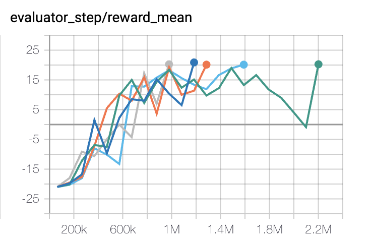
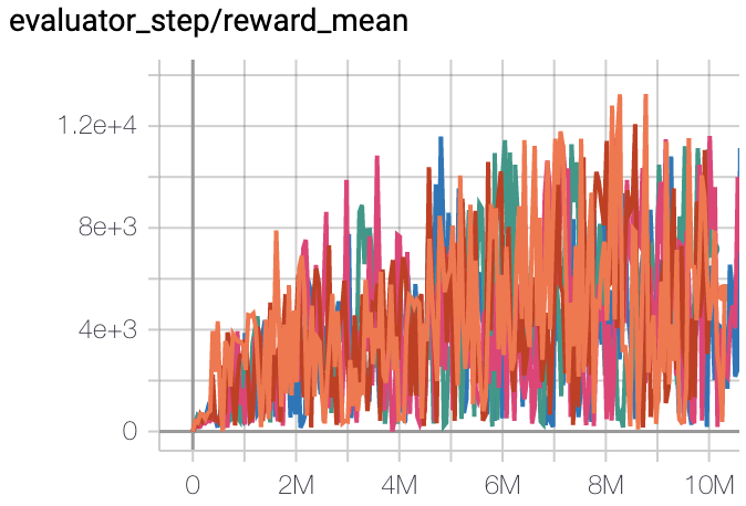
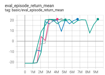
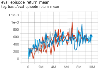
基准测试
环境 |
最佳平均奖励 |
评估结果 |
配置链接 |
比较 |
|---|---|---|---|---|
Pong
(PongNoFrameskip-v4)
|
20 |
|
IMPALA paper shallow 200M (20.4)
|
|
Qbert
(QbertNoFrameskip-v4)
|
13175 |
|
IMPALA paper shallow 200M (18901)
|
|
SpaceInvaders
(SpaceInvadersNoFrame skip-v4)
|
977 |

|
IMPALA paper shallow 200M (1726)
|
|
Pong(In new pipeline)
(Pong skip-v4)
|
21 |
|
IMPALA paper shallow 200M (20.4)
|
|
SpaceInvaders(In new pipeline)
(SpaceInvadersNoFrame skip-v4)
|
1006 |
|
IMPALA paper shallow 200M (1726)
|
附注:
上述结果是通过在五个不同的随机种子(0, 1, 2, 3, 4)上运行相同的配置获得的
带有新管道后缀的环境是使用新的训练过程进行训练的。新的训练过程更加简洁明了,数据收集速度更快。
对于像IMPALA这样的离散动作空间算法,通常使用Atari环境集进行测试(包括子环境Pong),并且Atari环境通常通过最高平均奖励训练10M
env_step来评估。有关Atari的更多详细信息,请参阅 Atari Env Tutorial 。
参考
Lasse Espeholt, Hubert Soyer, Remi Munos, Karen Simonyan, Volodymir Mnih, Tom Ward, Yotam Doron, Vlad Firoiu, Tim Harley, Iain Dunning, Shane Legg, Koray Kavukcuoglu: “IMPALA: 可扩展的分布式深度强化学习与重要性加权演员-学习者架构”, 2018; arXiv:1802.01561. https://arxiv.org/abs/1802.01561
其他公共实现
[Facebook torchbeast](https://github.com/facebookresearch/torchbeast)