医疗案例中的反事实分析

在这个例子中，我们研究了一个情况，即我们想要对已经发生的事件提出反事实问题。我们关注一个与视力问题相关的远程医疗示例，其中我们知道三个观察变量的因果结构，并且我们想要提出基于“如果我遵循了远程医疗应用程序提出的不同方法，会发生什么？”类型的反事实问题。

更具体地说，我们考虑以下情况。Alice因为眼睛干涩严重，决定使用一个远程医疗在线平台，因为她无法在她居住的地方看眼科医生。她经历了报告她的医疗历史的步骤，这揭示了Alice是否有罕见的过敏反应，平台最终推荐了她两种可能的眼药水，成分略有不同（'选项1'和'选项2'）。Alice在网上快速搜索了一下，发现选项1有很多正面评价。然而，她决定使用选项2，因为她的母亲过去也使用过，并且效果很好。几天后，Alice的视力变得好多了，她的症状开始消失。然而，她非常好奇如果她使用了非常受欢迎的选项1，或者甚至什么都不做，会发生什么。

该平台为用户提供了提出反事实问题的可能性，只要他们报告了他们所遵循选项的结果。

数据

我们有一个包含三个观察变量的数据库：一个从0到1的连续变量，表示视力质量（'Vision'），一个二元变量，表示患者是否有罕见病症（即过敏）（'Condition'），以及一个分类变量（'Treatment'），可以取三个值（0：'什么都不做'，1：'选项1'或2：'选项2'）。数据看起来像这样：

import pandas as pd

medical_data = pd.read_csv('patients_database.csv')
medical_data.head()

	条件	治疗	视力
0	0	2	0.111728
1	0	0	0.191516
2	0	2	0.163924
3	0	1	0.886563
4	0	1	0.761090

medical_data.iloc[0:100].plot(figsize=(15, 10))

<Axes: >

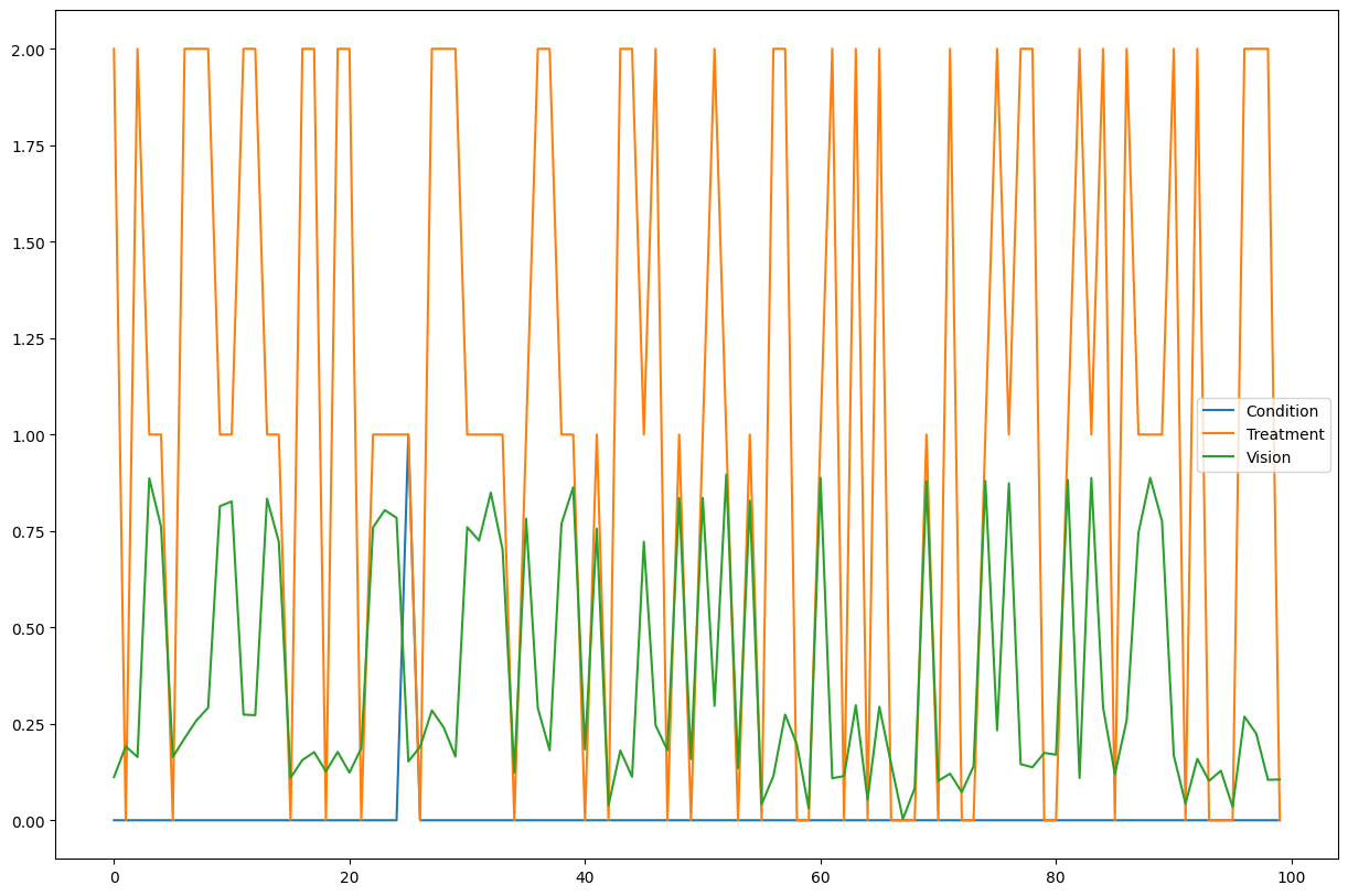
数据集反映了患者在根据是否患有罕见病症而选择三种治疗方案之一后的视力情况。请注意，数据集中没有关于患者治疗前原始视力的信息（即视力变量的噪声部分）。正如我们将在下面看到的，只要我们有一个后非线性模型（例如ANM），反事实算法就能够恢复这部分视力噪声。用于生成数据的结构因果模型在附录中有详细说明。这三个观察到的节点中的每一个都有一个内在的噪声，这是未被观察到的。

图的建模

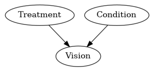
我们知道治疗节点和条件节点导致了视觉，但我们不知道结构因果模型。然而，我们可以从观察到的数据中学习它，特别是只要不违反后非线性模型假设，我们就能够为特定观察重建噪声。我们假设这个图正确地表示了因果关系，并且假设没有隐藏的混杂因素（因果充分性）。基于给定的图和数据，我们可以拟合因果模型并开始回答反事实问题。

import networkx as nx
import dowhy.gcm as gcm
from dowhy.utils import plot

causal_model = gcm.InvertibleStructuralCausalModel(nx.DiGraph([('Treatment', 'Vision'), ('Condition', 'Vision')]))
gcm.auto.assign_causal_mechanisms(causal_model, medical_data)

plot(causal_model.graph)

gcm.fit(causal_model, medical_data)

Fitting causal mechanism of node Condition: 100%|██████████| 3/3 [00:00<00:00, 30.13it/s]

可选地，我们现在也可以评估拟合的因果模型：

print(gcm.evaluate_causal_model(causal_model, medical_data))

Evaluating causal mechanisms...: 100%|██████████| 3/3 [00:00<00:00, 3583.85it/s]
Test permutations of given graph: 100%|██████████| 6/6 [00:00<00:00, 89.40it/s]

Evaluated the performance of the causal mechanisms and the invertibility assumption of the causal mechanisms and the overall average KL divergence between generated and observed distribution and the graph structure. The results are as follows:

==== Evaluation of Causal Mechanisms ====
The used evaluation metrics are:
- KL divergence (only for root-nodes): Evaluates the divergence between the generated and the observed distribution.
- Mean Squared Error (MSE): Evaluates the average squared differences between the observed values and the conditional expectation of the causal mechanisms.
- Normalized MSE (NMSE): The MSE normalized by the standard deviation for better comparison.
- R2 coefficient: Indicates how much variance is explained by the conditional expectations of the mechanisms. Note, however, that this can be misleading for nonlinear relationships.
- F1 score (only for categorical non-root nodes): The harmonic mean of the precision and recall indicating the goodness of the underlying classifier model.
- (normalized) Continuous Ranked Probability Score (CRPS): The CRPS generalizes the Mean Absolute Percentage Error to probabilistic predictions. This gives insights into the accuracy and calibration of the causal mechanisms.
NOTE: Every metric focuses on different aspects and they might not consistently indicate a good or bad performance.
We will mostly utilize the CRPS for comparing and interpreting the performance of the mechanisms, since this captures the most important properties for the causal model.

--- Node Treatment
- The KL divergence between generated and observed distribution is 0.0.
The estimated KL divergence indicates an overall very good representation of the data distribution.

--- Node Condition
- The KL divergence between generated and observed distribution is 0.0.
The estimated KL divergence indicates an overall very good representation of the data distribution.

--- Node Vision
- The MSE is 0.003263619495320028.
- The NMSE is 0.1825934384257641.
- The R2 coefficient is 0.9666581502186975.
- The normalized CRPS is 0.10654769436589524.
The estimated CRPS indicates a very good model performance.

==== Evaluation of Invertible Functional Causal Model Assumption ====

--- The model assumption for node Vision is not rejected with a p-value of 0.3758057876871662 (after potential adjustment) and a significance level of 0.05.
This implies that the model assumption might be valid.

Note that these results are based on statistical independence tests, and the fact that the assumption was not rejected does not necessarily imply that it is correct. There is just no evidence against it.

==== Evaluation of Generated Distribution ====
The overall average KL divergence between the generated and observed distribution is 0.0
The estimated KL divergence indicates an overall very good representation of the data distribution.

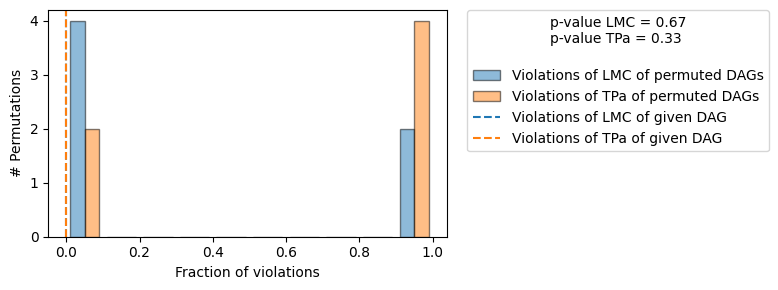
==== Evaluation of the Causal Graph Structure ====
+-------------------------------------------------------------------------------------------------------+
|                                         Falsification Summary                                         |
+-------------------------------------------------------------------------------------------------------+
| The given DAG is not informative because 2 / 6 of the permutations lie in the Markov                  |
| equivalence class of the given DAG (p-value: 0.33).                                                   |
| The given DAG violates 0/2 LMCs and is better than 33.3% of the permuted DAGs (p-value: 0.67).        |
| Based on the provided significance level (0.2) and because the DAG is not informative,                |
| we do not reject the DAG.                                                                             |
+-------------------------------------------------------------------------------------------------------+

==== NOTE ====
Always double check the made model assumptions with respect to the graph structure and choice of causal mechanisms.
All these evaluations give some insight into the goodness of the causal model, but should not be overinterpreted, since some causal relationships can be intrinsically hard to model. Furthermore, many algorithms are fairly robust against misspecifications or poor performances of causal mechanisms.

这证实了我们因果模型的准确性。

现在回到我们最初的问题，让我们加载Alice的数据，她恰好有一种罕见的过敏症（Condition = 1）。

specific_patient_data = pd.read_csv('newly_come_patients.csv')
specific_patient_data.head()

	条件	治疗	视力
0	1	2	0.883874

回答Alice的反事实查询

在我们想要检查如果某个事件没有发生或以不同方式发生时的假设结果的情况下，我们采用基于结构因果模型的所谓反事实逻辑。给定：- 我们知道Alice的治疗选择是选项2。- Alice有罕见的过敏（Condition=1）。- Alice在治疗选项2后的视力是0.78（Vision=0.78）。- 我们能够根据学习到的结构因果模型恢复噪声。

我们现在可以检查如果治疗节点不同，她的视力的反事实结果。在下面，我们看看如果Alice没有接受治疗（Treatment=0）和如果她接受了另一种眼药水（Treatment=1）时，她的视力的反事实值。

counterfactual_data1 = gcm.counterfactual_samples(causal_model,
                                                  {'Treatment': lambda x: 1},
                                                  observed_data = specific_patient_data)

counterfactual_data2 = gcm.counterfactual_samples(causal_model,
                                                  {'Treatment': lambda x: 0},
                                                  observed_data = specific_patient_data)


import matplotlib.pyplot as plt

df_plot2 = pd.DataFrame()
df_plot2['Vision after option 2'] = specific_patient_data['Vision']
df_plot2['Counterfactual vision (option 1)'] = counterfactual_data1['Vision']
df_plot2['Counterfactual vision (No treatment)'] = counterfactual_data2['Vision']

df_plot2.plot.bar(title="Counterfactual outputs")
plt.xlabel('Alice')
plt.ylabel('Eyesight quality')
plt.legend()

<matplotlib.legend.Legend at 0x7fc783d740a0>

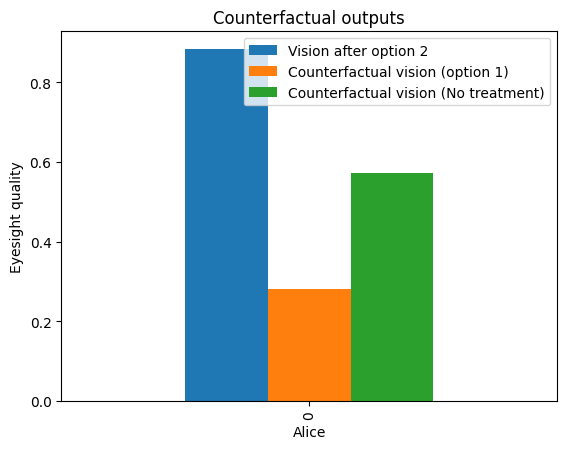
我们在这里看到的是，如果Alice选择了选项1而不是选项2，她的视力会比选择选项2时变得更差。因此，她意识到她在病史中报告的罕见情况（Condition=1）可能是导致她对流行的选项1产生过敏反应的原因。Alice还能够看到，如果她没有采取任何推荐的选项，她的视力会比她选择的选项2更差（变量Vision的相对值更小）。

附录：远程应用程序内部使用的内容。患者日志的数据生成

这里我们描述了加性噪声模型的SCM \(f_{p1, p2}\)：\(Vision = N_V + f_{p1, p2}(Treatment, Condition)\)。我们对三个观察变量\(N_T, N_C\)和\(N_V\)的内在加性噪声进行采样。然后，目标变量Vision是加性噪声\(N_V\)加上其输入节点的函数，如下所述。

\(Treatment = N_T\) ~ 0 , 1 或 2，概率分别为 33%：33% 的用户不做任何操作，33% 选择选项 1，33% 选择选项 2。这与患者是否患有罕见病症无关。

\(Condition = N_C\) ~ Bernoulli(0.01) : 患者是否患有罕见病症

$Vision = N_V + f_{p1, p2}(Treatment, Condition) = N_V - P_1(1 - Condition)(1-Treatment)(2-Treatment) + 2P_2(1-Condition)Treatment(2-Treatment) + P_2(1-Condition)(3-Treatment)(1-Treatment)Treatment - 2P_2 Condition Treatment(2-Treatment) - P_2 Condition(3-Treatment)(1-Treatment)Treatment $ 患者的视力，其中：

\(P_1\) 是一个常数，表示如果患者没有罕见病症且未接受任何药物治疗，原始视力将会减少的程度。

\(P_2\) 是一个常数，根据患者是否患有该病症以及他们将使用的滴剂类型，原始视力将相应增加或减少。更具体地说：

如果条件 = 0 且 处理 = 1 那么 视力 = N_V + P_2

如果条件 = 0 且 处理 = 2 那么 视力 = N_V - P_2

如果条件 = 1 且 治疗 = 1 那么 视力 = N_V - P_2

如果条件 = 1 且 处理 = 2 那么 视力 = N_V + P_2

如果条件 = 0 且处理 = 0，则视觉 = N_V - P_1

如果条件 = 1 且处理 = 0，则视觉 = N_V - P3

注意 对于反事实陈述，分配的功能因果模型必须相对于噪声是可逆的（例如，加性噪声模型）。或者，用户也可以指定真实模型和真实噪声。

对于像具有条件（Condition=1，其概率仅为1%）这样的罕见事件，需要大量的样本来训练模型，以准确反映这些罕见事件。这就是为什么我们在这里使用了10000个样本来生成患者数据库。

from scipy.stats import bernoulli, norm, uniform
import numpy as np
from random import randint

n_unobserved = 10000
unobserved_data = {
   'N_T': np.array([randint(0, 2) for p in range(n_unobserved)]),
   'N_vision': np.random.uniform(0.4, 0.6, size=(n_unobserved,)),
   'N_C': bernoulli.rvs(0.01, size=n_unobserved)
}
P_1 = 0.2
P_2 = 0.15

def create_observed_medical_data(unobserved_data):
    observed_medical_data = {}
    observed_medical_data['Condition'] = unobserved_data['N_C']
    observed_medical_data['Treatment'] = unobserved_data['N_T']
    observed_medical_data['Vision'] = unobserved_data['N_vision'] + (-P_1)*(1 - observed_medical_data['Condition'])*(1 - observed_medical_data['Treatment'])*(2 - observed_medical_data['Treatment']) + (2*P_2)*(1 - observed_medical_data['Condition'])*(observed_medical_data['Treatment'])*(2 - observed_medical_data['Treatment']) + (P_2)*(1 - observed_medical_data['Condition'])*(observed_medical_data['Treatment'])*(1 - observed_medical_data['Treatment'])*(3 - observed_medical_data['Treatment']) + 0*(observed_medical_data['Condition'])*(1 - observed_medical_data['Treatment'])*(2 - observed_medical_data['Treatment']) + (-2*P_2)*(unobserved_data['N_C'])*(observed_medical_data['Treatment'])*(2 - observed_medical_data['Treatment']) + (-P_2)*(observed_medical_data['Condition'])*(observed_medical_data['Treatment'])*(1 - observed_medical_data['Treatment'])*(3 - observed_medical_data['Treatment'])
    return pd.DataFrame(observed_medical_data)

medical_data = create_observed_medical_data(unobserved_data)

生成Alice的数据：她的初始视觉的随机噪声，Condition=1（因为她有罕见的过敏）和她最初决定采取Treatment=2（眼药水选项2）。

num_samples = 1
original_vision = np.random.uniform(0.4, 0.6, size=num_samples)
def generate_specific_patient_data(num_samples):
    return create_observed_medical_data({
    'N_T': np.full((num_samples,), 2),
    'N_C': bernoulli.rvs(1, size=num_samples),
    'N_vision': original_vision,
})

specific_patient_data = generate_specific_patient_data(num_samples)