分解性别工资差距#
在本笔记本中,我们研究了真实人口普查数据中性别工资差距有多少可以归因于女性和男性在教育或职业上的差异。我们使用了以下论文中的多重稳健因果变化归因方法:>Quintas-Martínez, V., Bahadori, M. T., Santiago, E., Mu, J. 和 Heckerman, D. “多重稳健因果变化归因”,第41届国际机器学习会议论文集,维也纳,奥地利。PMLR 235, 2024。
读取并准备数据#
我们将使用2015年当前人口调查(CPS)的数据。在应用与Chernozhukov等人(2018)相同的样本限制后,最终样本包含18,137名男性和14,382名女性就业个体。
[1]:
import pandas as pd

# Read and prepare data:
df = pd.read_csv('./cps2015.csv')

# LightGBM works best with integer encoding for categorical variables:
educ_int = {'lhs' : 0, 'hsg' : 1, 'sc' : 2, 'cg' : 3, 'ad' : 4}
df['education'] = pd.from_dummies(df[['lhs', 'hsg', 'sc', 'cg', 'ad']])
df['education'] = df['education'].replace(educ_int)

df = df[['female', 'education', 'occ2', 'wage', 'weight']]
df.columns = ['female', 'education', 'occupation', 'wage', 'weight']
df[['education', 'occupation']] = df[['education', 'occupation']].astype('category')

# We want to explain the change Male -> Female:
data_old, data_new = df.loc[df.female == 0], df.loc[df.female == 1]
因果模型#
要使用我们的因果变化归因方法,我们需要一个将结果(工资)和解释变量联系起来的因果模型。(实际上,该方法只需要知道一个因果顺序。)我们将使用以下DAG:
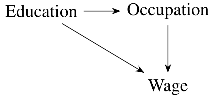
上面的DAG暗示了数据分布的以下因果马尔可夫分解:
这个分解的每个组成部分(DAG中每个节点给定其直接原因的分布)被称为因果机制。男性和女性之间工资边际分布的差异可能是由于每个因果机制的差异。我们的目标是解开每个机制对总变化的贡献。
在下面的代码中,我们定义了一个 dowhy.gcm 因果模型:
[2]:
import networkx as nx
import dowhy.gcm as gcm

dag = nx.DiGraph([('education', 'occupation'), ('occupation', 'wage'), ('education', 'wage')])
causal_model = gcm.ProbabilisticCausalModel(dag)
使用dowhy.gcm.distribution_change_robust实现#
首先,我们展示如何使用dowhy.gcm.distribution_change_robust函数计算因果变化归因度量(Shapley值)。
多重稳健因果变化归因方法基于回归和重加权方法的组合。在回归方法中,我们学习一个样本中节点与其父节点之间的依赖关系,然后使用另一个样本的数据来转移该节点的分布。在重加权方法中,我们对数据进行平均,给予那些与目标分布非常相似的观察值更多的权重。
默认情况下,dowhy.gcm.distribution_change_robust 使用线性回归和逻辑回归来学习回归函数和权重。这里,由于我们的数据集相当大,我们将使用更灵活的算法 HistGradientBoostingRegressor 和 HistGradientBoostingClassifier 来代替。
我们还使用IsotonicRegression来校准构成重加权方法权重的概率,这是在留出校准样本上进行的。这是可选的,但已证明在模拟中可以提高方法的性能。
最后,由于我们的数据集很大,我们将使用样本分割(而不是交叉拟合)。也就是说,我们将随机将数据分为训练集和评估集,在训练集中学习回归和权重,在评估集中使用回归和权重来计算最终的归因度量。
[3]:
from sklearn.ensemble import HistGradientBoostingRegressor, HistGradientBoostingClassifier
from sklearn.isotonic import IsotonicRegression
from dowhy.gcm.ml.classification import SklearnClassificationModelWeighted
from dowhy.gcm.ml.regression import SklearnRegressionModelWeighted
from dowhy.gcm.util.general import auto_apply_encoders, auto_fit_encoders, shape_into_2d

def make_custom_regressor():
    return SklearnRegressionModelWeighted(HistGradientBoostingRegressor(random_state = 0))

def make_custom_classifier():
    return SklearnClassificationModelWeighted(HistGradientBoostingClassifier(random_state = 0))

def make_custom_calibrator():
    return SklearnRegressionModelWeighted(IsotonicRegression(out_of_bounds = 'clip'))

gcm.distribution_change_robust(causal_model, data_old, data_new, 'wage', sample_weight = 'weight',
                               xfit = False, calib_size = 0.2,
                               regressor = make_custom_regressor,
                               classifier = make_custom_classifier,
                               calibrator = make_custom_calibrator)
Evaluating set functions...: 100%|██████████| 8/8 [00:02<00:00, 3.77it/s]
[3]:
{'education': 1.1321504485335492,
 'occupation': -2.0786979433836734,
 'wage': -6.809529336261436}
该函数返回一个字典,其中每个值是对应于键的因果机制的Shapley Value因果归因度量。(有关Shapley Values的正式定义,请参阅研究论文。)我们在本笔记本的最后部分对结果进行了更深入的解释。
手动实现(高级)#
其次,我们展示了如何更直接地使用类 dowhy.gcm.distribution_change_robust.ThetaC 来实现该方法,该类允许更高级的功能,包括通过高斯乘数自举法计算标准误差(见下文)。
[4]:
from sklearn.model_selection import StratifiedKFold, train_test_split

# Split data into train and test set:
X = df[['education', 'occupation']].values
y = df['wage'].values
T = df['female'].values
w = df['weight'].values

# To get the same train-test split:
kf = StratifiedKFold(n_splits = 2, shuffle = True, random_state = 0)
train_index, test_index = next(kf.split(X, T))

X_train, X_eval, y_train, y_eval, T_train, T_eval = X[train_index], X[test_index], y[train_index], y[test_index], T[train_index], T[test_index]
w_train, w_eval = w[train_index], w[test_index]

X_calib, X_train, _, y_train, T_calib, T_train, w_calib, w_train = train_test_split(X_train, y_train, T_train, w_train,
                                                                                    train_size = 0.2, stratify = T_train, random_state = 0)
[5]:
import itertools
from dowhy.gcm.distribution_change_robust import ThetaC
import numpy as np
from math import comb

# All combinations of 0s and 1s, needed for Shapley Values:
all_combos = [list(i) for i in itertools.product([0, 1], repeat=3)]
all_combos_minus1 = [list(i) for i in itertools.product([0, 1], repeat=2)]

# Dictionary to store the multiply-robust scores, will be used later for bootstrap:
scores = {}

# Here we compute the theta^c parameters that make up the Shapley Values (see paper):
for C in all_combos:
    scores[''.join(str(x) for x in C)] = ThetaC(C).est_scores(
        X_eval,
        y_eval,
        T_eval,
        X_train,
        y_train,
        T_train,
        w_eval=w_eval,
        w_train=w_train,
        X_calib=X_calib,
        T_calib=T_calib,
        w_calib=w_calib,
        regressor = make_custom_regressor,
        classifier = make_custom_classifier,
        calibrator = make_custom_calibrator)

# This function combines the theta^c parameters to obtain Shapley values:
w_sort = np.concatenate((w_eval[T_eval==0], w_eval[T_eval==1])) # Order weights in same way as scores

def compute_attr_measure(res_dict, path=False):
    # Alternative to Shapley Value: along-a-causal-path (see paper)
    if path:
        path = np.zeros(3)
        path[0] = np.average(res_dict['100'], weights=w_sort) - np.average(res_dict['000'], weights=w_sort)
        path[1] = np.average(res_dict['110'], weights=w_sort) - np.average(res_dict['100'], weights=w_sort)
        path[2] = np.average(res_dict['111'], weights=w_sort) - np.average(res_dict['110'], weights=w_sort)
        return path

    # Shapley values:
    else:
        shap = np.zeros(3)
        for k in range(3):
            sv = 0.0
            for C in all_combos_minus1:
                C1 = np.insert(C, k, True)
                C0 = np.insert(C, k, False)
                chg = (np.average(res_dict[''.join(map(lambda x : str(int(x)), C1))], weights=w_sort) -
                       np.average(res_dict[''.join(map(lambda x : str(int(x)), C0))], weights=w_sort))
                sv += chg/(3*comb(2, np.sum(C)))
            shap[k] = sv
        return shap

shap = compute_attr_measure(scores, path=False)
shap # Should coincide with the above
[5]:
array([ 1.13215045, -2.07869794, -6.80952934])
由于多重稳健性特性,我们可以使用一种快速形式的自举法来计算标准误差,这种方法不需要在每次自举迭代时重新估计回归和权重。相反,我们只需使用独立同分布的正态分布(0, 1)随机数重新加权数据。
[6]:
w_sort = np.concatenate((w_eval[T_eval==0], w_eval[T_eval==1])) # Order weights in same way as scores

def mult_boot(res_dict, Nsim=1000, path=False):
    thetas = np.zeros((8, Nsim))
    attr = np.zeros((3, Nsim))
    for s in range(Nsim):
        np.random.seed(s)
        new_scores = {}
        for k, x in res_dict.items():
            new_scores[k] = x + np.random.normal(0,1, X_eval.shape[0])*(x - np.average(x, weights=w_sort))
        thetas[:, s] = np.average(np.array([x for k, x in new_scores.items()]), axis=1, weights=w_sort)
        attr[:, s] = compute_attr_measure(new_scores, path)
    return np.std(attr, axis=1)

shap_se = mult_boot(scores, path=False)
shap_se
[6]:
array([0.34144275, 0.35141792, 0.35805933])
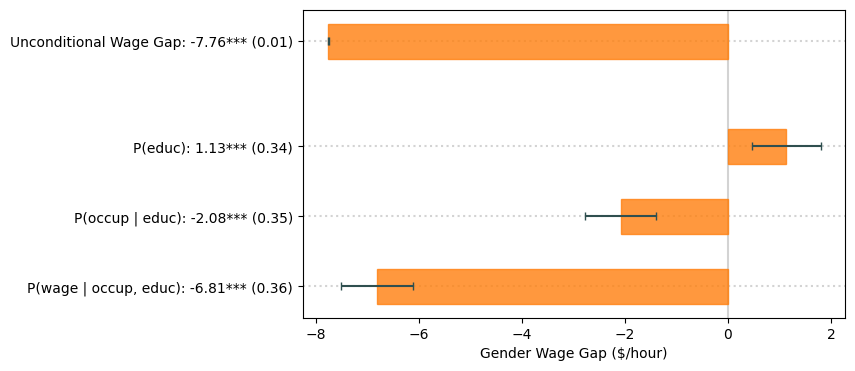
我们可以在图表中直观地展示结果,如论文中所示:
[7]:
from scipy.stats import norm
from statsmodels.stats.weightstats import DescrStatsW
from matplotlib.patches import Rectangle
import matplotlib.pyplot as plt

# Significance stars:
def star(est, se):
    if np.abs(est/se)<norm.ppf(.95): # 10%
        return ''
    elif np.abs(est/se)<norm.ppf(.975): # 5%
        return '*'
    elif np.abs(est/se)<norm.ppf(.995): # 1%
        return '**'
    else:
        return '***'

# Unconditional wage gap:
stats0 = DescrStatsW(y_eval[T_eval==0], weights=w_eval[T_eval==0], ddof=0)
stats1 = DescrStatsW(y_eval[T_eval==1], weights=w_eval[T_eval==1], ddof=0)

wagegap = (stats1.mean - stats0.mean)
wagegap_se = np.sqrt(stats1.std_mean**2 + stats0.std_mean**2)

# Plot
nam = ["P(educ)", "P(occup | educ)", "P(wage | occup, educ)"]

crit = norm.ppf(.975) # 5% critical value (for error bars)
stars = [star(est, se) for est, se in zip(shap, shap_se)]
fig, ax = plt.subplots()
ax.axvline(x = 0, color='lightgray', zorder=0)
fig.set_size_inches(7, 4)

color = 'C1'
ax.add_patch(Rectangle((0, 4.75), width = wagegap, height = 0.5, color=color, alpha=0.8))
ax.plot((wagegap-crit*wagegap_se, wagegap+crit*wagegap_se,), (5.0, 5.0), color='darkslategray', marker='|', solid_capstyle='butt')
ax.axhline(y = 5.0, color='lightgray', linestyle='dotted', zorder=0)

for i in range(len(shap)):
    pos = (shap[i], 3-i+0.25) if shap[i] < 0 else (0, 3-i+0.25)
    width = np.abs(shap[i])
    ax.add_patch(Rectangle(pos, width = width, height = 0.5, color=color, alpha=0.8))
    ax.axhline(y = 3+0.5-i, color='lightgray', linestyle='dotted', zorder=0)
    ax.plot((shap[i]-crit*shap_se[i], shap[i]+crit*shap_se[i]), (3-i+0.5, 3-i+0.5), color='darkslategray', marker='|', solid_capstyle='butt')
plt.yticks([5.0] + [3+0.5-i for i in range(3)], [f'Unconditional Wage Gap: {wagegap:.2f}*** ({wagegap_se:.2f})'] +
           ["{}: {:.2f}{} ({:.2f})".format(nam[i], shap[i], stars[i], shap_se[i]) for i in range(3)])
plt.xlabel('Gender Wage Gap ($/hour)')
plt.show()
解释#
首先,注意到 \(P(\mathtt{educ})\)、\(P(\mathtt{occup} \mid \mathtt{educ})\) 和 \(P(\mathtt{wage} \mid \mathtt{occup}, \mathtt{educ})\) 的 Shapley 值加起来等于总效应。
其次,\(P(\mathtt{educ})\) 的 Shapley 值为正且具有统计显著性。解释这一指标的一种方式是,如果男性和女性仅在 \(P(\mathtt{educ})\) 上存在差异(但他们的其他因果机制相同),女性平均每小时收入将比男性多 \$1.13。相反,\(P(\mathtt{educ} \mid \mathtt{educ})\) 的 Shapley 值为负,具有统计显著性且幅度大于第一个 Shapley 值,因此抵消了教育差异的影响。这些效应衡量了两点:1. 男性和女性之间的因果机制有多大差异?2. 因果机制对结果有多重要?
第三,大部分无条件的工资差距归因于因果机制 \(P(\mathtt{wage} \mid \mathtt{occup}, \mathtt{educ})\)。这可以通过多种方式解释:1. 未解释的变异:可能存在我们没有测量的其他相关变量,这些变量被包含在 \(P(\mathtt{wage} \mid \mathtt{occup}, \mathtt{educ})\) 中。例如,男性和女性之间可能存在经验差异,而这些差异在CPS数据中没有被测量。请注意,这不会对我们其他Shapley值的结果产生偏差,因为经验并不是教育或职业的直接原因。2. 结构差异:另一种解释是,由于某种原因(可能是歧视,也可能不是),具有相同可观察特征的男性和女性的工资不同。
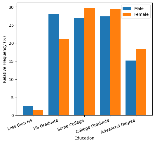
下面我们尝试通过一些图表来理解这一点。首先,注意到女性往往比男性拥有更高的教育水平。作为比较,大学毕业生平均每小时比高中毕业生多赚12.60美元。
[8]:
w0, w1 = w_eval[T_eval==0], w_eval[T_eval==1]

data_male_eval = pd.DataFrame({'education' : X_eval[:,0][T_eval==0],
                              'occupation' : X_eval[:,1][T_eval==0],
                              'wage' : y_eval[T_eval==0]})
data_female_eval = pd.DataFrame({'education' : X_eval[:,0][T_eval==1],
                              'occupation' : X_eval[:,1][T_eval==1],
                              'wage' : y_eval[T_eval==1]})

educ_names = {0 : 'Less than HS', 1 : 'HS Graduate', 2 : 'Some College', 3 : 'College Graduate', 4 : 'Advanced Degree'}
data_male_eval['education'] = data_male_eval['education'].replace(educ_names)
data_female_eval['education'] = data_female_eval['education'].replace(educ_names)

cats_educ = [educ_names[i] for i in range(5)]

ind = np.arange(len(cats_educ))
share0, share1 = np.zeros(len(cats_educ)), np.zeros(len(cats_educ))
for i, c in enumerate(cats_educ):
    share0[i] = np.sum(w0*(data_male_eval['education'] == c))/np.sum(w0)*100
    share1[i] = np.sum(w1*(data_female_eval['education'] == c))/np.sum(w1)*100

fig = plt.figure()
fig.set_size_inches(6, 5)
plt.bar(ind, share0, 0.4, label='Male')
plt.bar(ind+0.4, share1, 0.4, label='Female')
plt.xticks(ind+0.2, cats_educ, rotation=20, ha='right')
plt.ylabel('Relative Frequency (%)')
plt.xlabel('Education')
plt.legend()
plt.show()

# College graduates vs. high school graduates
diff = (np.average(df[df['education'] == 3]['wage'], weights=df[df['education'] == 3]['weight']) -
        np.average(df[df['education'] == 1]['wage'], weights=df[df['education'] == 1]['weight']))
print(f"College vs. HS: {diff:.2f}")
College vs. HS: 12.60
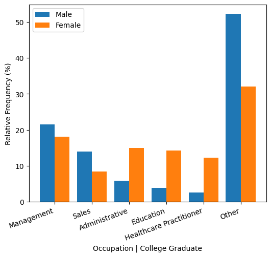
拥有大学学位的女性在行政、教育或医疗保健职业中更为普遍,而拥有大学学位的男性更可能从事管理或销售工作。相比之下,管理人员的平均工资比教育工作者每小时多16.66美元,比医疗保健从业者每小时多6.29美元。
然而,与此同时,存在一些无法通过教育或职业来解释的巨大差异。例如,女性大学毕业生经理的时薪比男性同行少13.77美元。
[9]:
occup_names= {1 : 'Management', 2 : 'Business/Finance', 3 : 'Computer/Math', 4 : 'Architecture/Engineering', 5 : 'Life/Physical/Social Science',
              6 : 'Community/Social Sevice', 7 : 'Legal', 8 : 'Education', 9 : 'Arts/Sports/Media', 10 : 'Healthcare Practitioner',
              11 : 'Healthcare Support', 12 : 'Protective Services', 13 : 'Food Preparation/Serving', 14 : 'Building Cleaning/Maintenance',
              15 : 'Personal Care', 16 : 'Sales', 17 : 'Administrative', 18: 'Farming/Fishing/Forestry', 19 : 'Construction/Mining',
              20 : 'Installation/Repairs', 21 : 'Production', 22 : 'Transportation'}
data_male_eval['occupation'] = data_male_eval['occupation'].replace(occup_names)
data_female_eval['occupation'] = data_female_eval['occupation'].replace(occup_names)

cats_occu = ['Management', 'Sales', 'Administrative', 'Education', 'Healthcare Practitioner', 'Other']

ind = np.arange(len(cats_occu))
share0, share1 = np.zeros(len(cats_occu)), np.zeros(len(cats_occu))
for i, c in enumerate(cats_occu[:-1]):
    share0[i] = np.sum(w0*((data_male_eval['occupation'] == c) & (data_male_eval['education'] ==
                                               'College Graduate')))/np.sum(w0 * (data_male_eval['education'] ==
                                               'College Graduate'))*100
    share1[i] = np.sum(w1*((data_female_eval['occupation'] == c) & (data_female_eval['education'] ==
                                               'College Graduate')))/np.sum(w1 * (data_female_eval['education'] ==
                                               'College Graduate'))*100
share0[-1] = np.sum(w0*((~data_male_eval['occupation'].isin(cats_occu[:-1])) & (data_male_eval['education'] ==
                                               'College Graduate')))/np.sum(w0 * (data_male_eval['education'] ==
                                               'College Graduate'))*100
share1[-1] = np.sum(w1*((~data_female_eval['occupation'].isin(cats_occu[:-1])) & (data_female_eval['education'] ==
                                               'College Graduate')))/np.sum(w1 * (data_female_eval['education'] ==
                                               'College Graduate'))*100

fig = plt.figure()
fig.set_size_inches(6, 5)
plt.bar(ind, share0, 0.4, label='Male')
plt.bar(ind+0.4, share1, 0.4, label='Female')
plt.xticks(ind+0.2, cats_occu, rotation=20, ha='right')
plt.ylabel('Relative Frequency (%)')
plt.xlabel('Occupation | College Graduate')
plt.legend()
plt.show()

# Managers vs. Education
diff = (np.average(df[df['occupation'] == 1]['wage'], weights=df[df['occupation'] == 1]['weight']) -
        np.average(df[df['occupation'] == 8]['wage'], weights=df[df['occupation'] == 8]['weight']))
print(f"Management vs. Education: {diff:.2f}")

# Managers vs. Healthcare
diff = (np.average(df[df['occupation'] == 1]['wage'], weights=df[df['occupation'] == 1]['weight']) -
        np.average(df[df['occupation'] == 10]['wage'], weights=df[df['occupation'] == 10]['weight']))
print(f"Management vs. Healthcare: {diff:.2f}")

# Female vs. Male College Managers
diff = (np.average(data_female_eval[np.logical_and(data_female_eval['occupation'] == 'Management', data_female_eval['education'] == 'College Graduate')]['wage'],
                   weights=w1[np.logical_and(data_female_eval['occupation'] == 'Management', data_female_eval['education'] == 'College Graduate')]) -
        np.average(data_male_eval[np.logical_and(data_male_eval['occupation'] == 'Management', data_male_eval['education'] == 'College Graduate')]['wage'],
                   weights=w0[np.logical_and(data_male_eval['occupation'] == 'Management', data_male_eval['education'] == 'College Graduate')]))
print(f"Female vs. Male College Managers: {diff:.2f}")
Management vs. Education: 16.66
Management vs. Healthcare: 6.29
Female vs. Male College Managers: -13.77
[ ]: