生成集群图

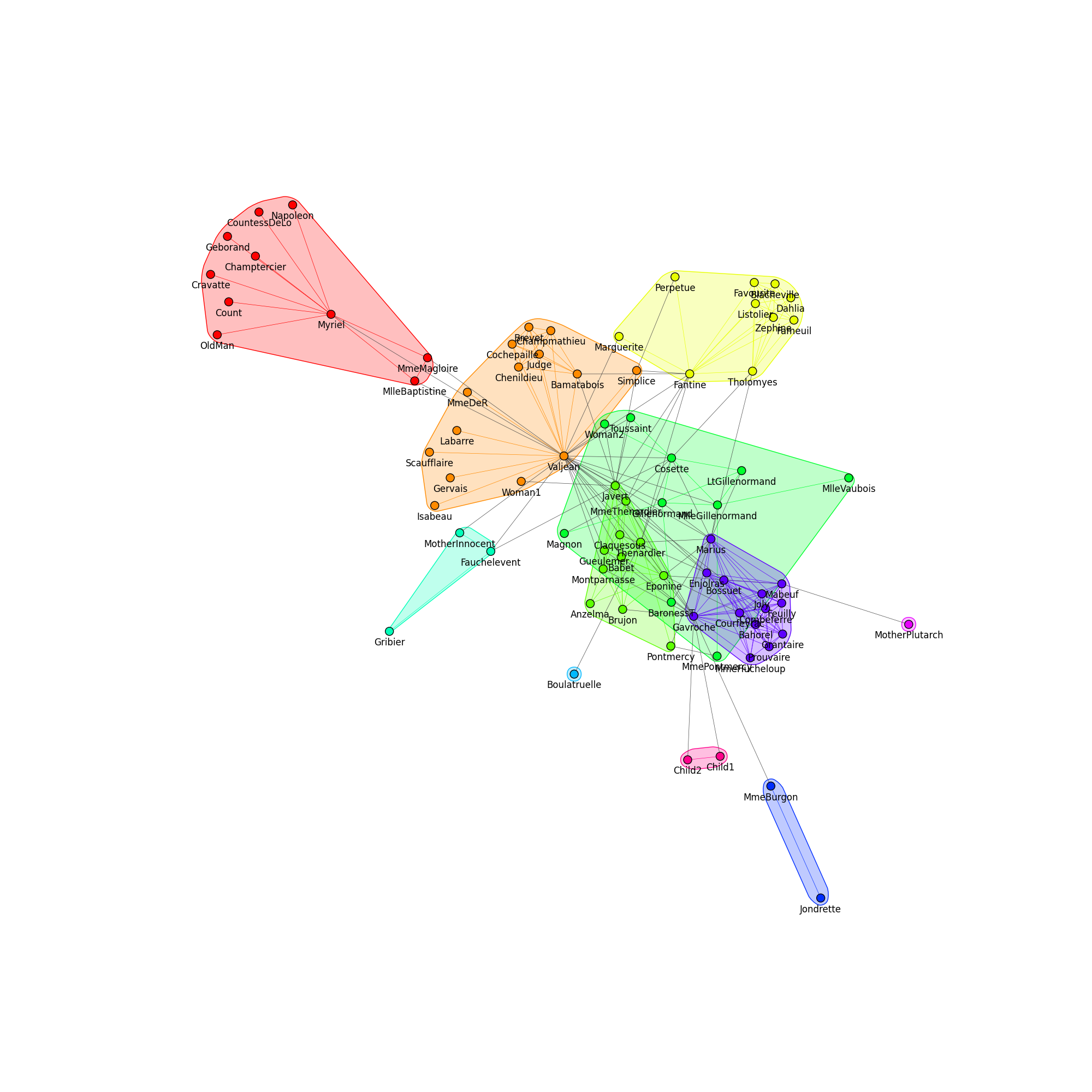
这个例子展示了如何在图中找到社区，然后使用igraph.clustering.VertexClustering将每个社区收缩为单个节点。在本教程中，我们将使用Donald Knuth的《悲惨世界》网络，它展示了小说《悲惨世界》中角色的共同出现情况。

import igraph as ig
import matplotlib.pyplot as plt

我们首先从文件中加载图。包含此网络的文件可以在这里下载。

g = ig.load("./lesmis/lesmis.gml")

现在我们已经在内存中有了一个图，我们可以使用 igraph.Graph.community_edge_betweenness() 来生成社区，将顶点分离成 集群。（有关仅可视化社区的更集中教程，请查看 Communities）。

communities = g.community_edge_betweenness()

对于绘图，将社区转换为VertexClustering非常方便：

communities = communities.as_clustering()

我们也可以轻松打印出每个社区的成员：

for i, community in enumerate(communities):
    print(f"Community {i}:")
    for v in community:
        print(f"\t{g.vs[v]['label']}")

Community 0:
        Myriel
        Napoleon
        MlleBaptistine
        MmeMagloire
        CountessDeLo
        Geborand
        Champtercier
        Cravatte
        Count
        OldMan
Community 1:
        Labarre
        Valjean
        MmeDeR
        Isabeau
        Gervais
        Bamatabois
        Simplice
        Scaufflaire
        Woman1
        Judge
        Champmathieu
        Brevet
        Chenildieu
        Cochepaille
Community 2:
        Marguerite
        Tholomyes
        Listolier
        Fameuil
        Blacheville
        Favourite
        Dahlia
        Zephine
        Fantine
        Perpetue
Community 3:
        MmeThenardier
        Thenardier
        Javert
        Pontmercy
        Eponine
        Anzelma
        Gueulemer
        Babet
        Claquesous
        Montparnasse
        Brujon
Community 4:
        Cosette
        Woman2
        Gillenormand
        Magnon
        MlleGillenormand
        MmePontmercy
        MlleVaubois
        LtGillenormand
        BaronessT
        Toussaint
Community 5:
        Fauchelevent
        MotherInnocent
        Gribier
Community 6:
        Boulatruelle
Community 7:
        Jondrette
        MmeBurgon
Community 8:
        Gavroche
        Marius
        Mabeuf
        Enjolras
        Combeferre
        Prouvaire
        Feuilly
        Courfeyrac
        Bahorel
        Bossuet
        Joly
        Grantaire
        MmeHucheloup
Community 9:
        MotherPlutarch
Community 10:
        Child1
        Child2

最后我们可以继续绘制图表。为了使每个社区突出，我们使用igraph调色板设置“社区颜色”：

num_communities = len(communities)
palette1 = ig.RainbowPalette(n=num_communities)
for i, community in enumerate(communities):
    g.vs[community]["color"] = i
    community_edges = g.es.select(_within=community)
    community_edges["color"] = i

我们可以使用一个巧妙的小技巧将标签移动到顶点下方 ;-)

g.vs["label"] = ["\n\n" + label for label in g.vs["label"]]

最后，我们可以绘制社区：

fig1, ax1 = plt.subplots()
ig.plot(
    communities,
    target=ax1,
    mark_groups=True,
    palette=palette1,
    vertex_size=15,
    edge_width=0.5,
)
fig1.set_size_inches(20, 20)

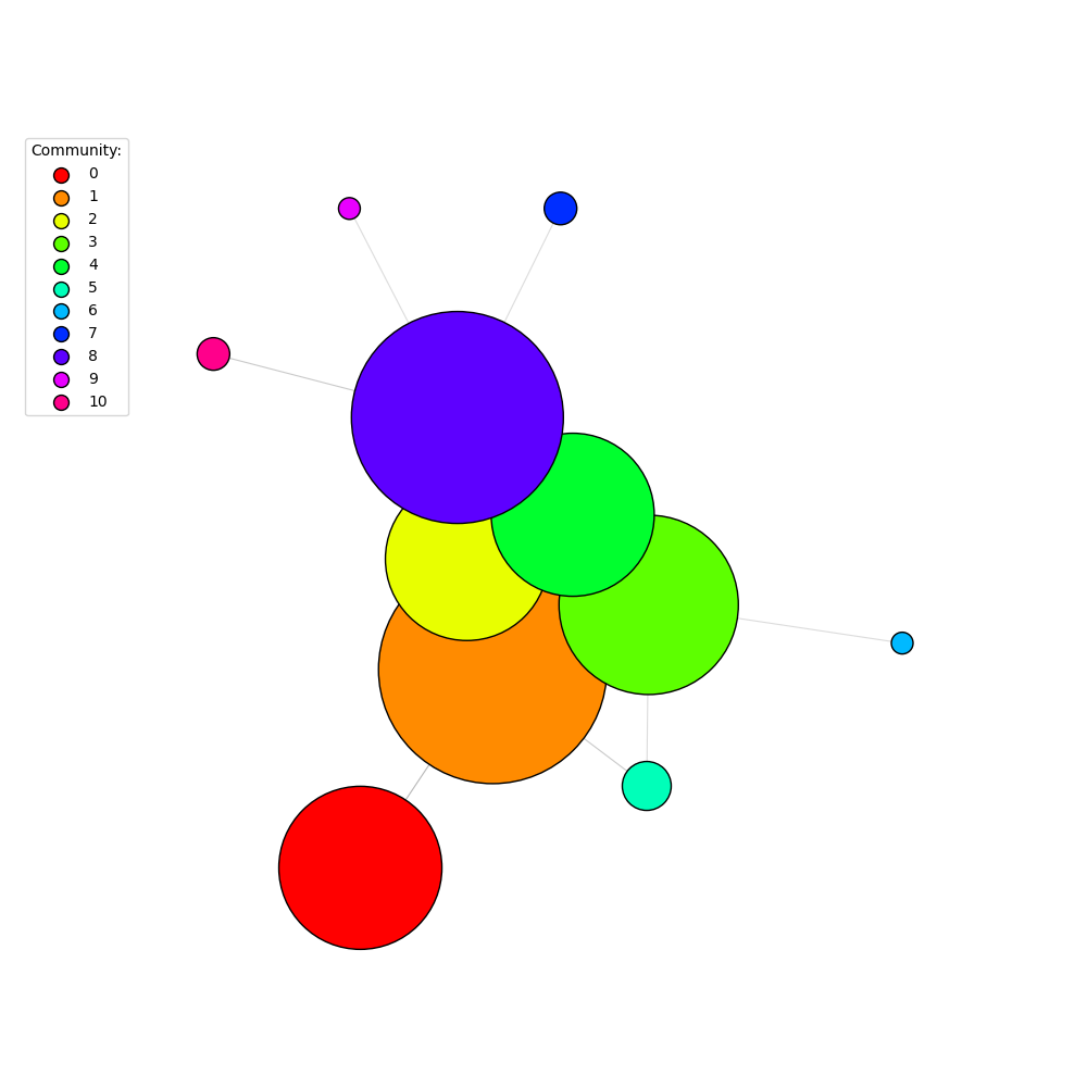
现在让我们尝试将信息压缩，仅使用一个顶点来代表每个社区。我们首先为原始图中的每个节点定义x、y和size属性：

layout = g.layout_kamada_kawai()
g.vs["x"], g.vs["y"] = list(zip(*layout))
g.vs["size"] = 15
g.es["size"] = 15

然后我们可以生成将每个社区压缩为单个“复合”顶点的集群图，使用 igraph.VertexClustering.cluster_graph():

cluster_graph = communities.cluster_graph(
    combine_vertices={
        "x": "mean",
        "y": "mean",
        "color": "first",
        "size": "sum",
    },
    combine_edges={
        "size": "sum",
    },
)

注意

我们取了x和y值的平均值，以便聚类图中的节点位于原始聚类的质心。

注意

mean, first, 和 sum 都是内置的聚合函数， 还有 prod, median, max, min, last, random。 你也可以定义自己的自定义聚合函数，这些函数接收一个 列表并返回一个代表组合属性值的单个元素。有关 igraph 收缩的更多详细信息，请参阅 igraph.GraphBase.contract_vertices()。

最后，我们可以为集群分配颜色并绘制集群图，包括一个图例以使内容清晰：

palette2 = ig.GradientPalette("gainsboro", "black")
g.es["color"] = [palette2.get(int(i)) for i in ig.rescale(cluster_graph.es["size"], (0, 255), clamp=True)]

fig2, ax2 = plt.subplots()
ig.plot(
    cluster_graph,
    target=ax2,
    palette=palette1,
    # set a minimum size on vertex_size, otherwise vertices are too small
    vertex_size=[max(20, size) for size in cluster_graph.vs["size"]],
    edge_color=g.es["color"],
    edge_width=0.8,
)

# Add a legend
legend_handles = []
for i in range(num_communities):
    handle = ax2.scatter(
        [], [],
        s=100,
        facecolor=palette1.get(i),
        edgecolor="k",
        label=i,
    )
    legend_handles.append(handle)

ax2.legend(
    handles=legend_handles,
    title='Community:',
    bbox_to_anchor=(0, 1.0),
    bbox_transform=ax2.transAxes,
)

fig2.set_size_inches(10, 10)