BiTCN

%load_ext autoreload
%autoreload 2

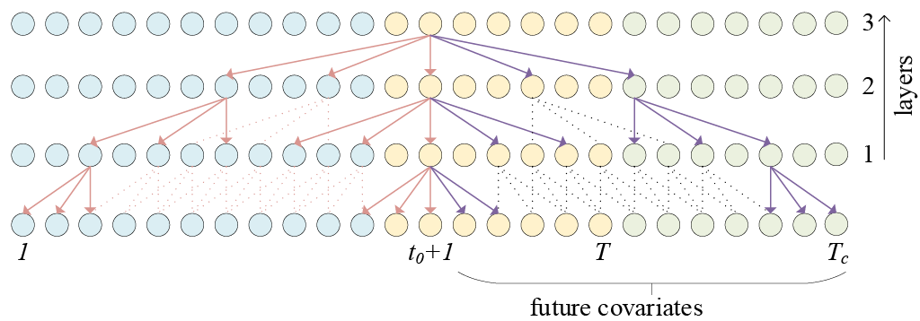
双向时间卷积网络（BiTCN）是一种基于两个时间卷积网络（TCNs）的预测架构。第一个网络（“前向”）编码时间序列的未来协变量，而第二个网络（“后向”）编码过去的观测值和协变量。这种方法可以保留序列数据的时间信息，并且在计算上比常见的RNN方法（如LSTM、GRU等）更加高效。与基于Transformer的方法相比，BiTCN具有较低的空间复杂度，即所需参数数量低几个数量级。

如果您寻求一个小模型（可训练参数少）且可调超参数较少（仅2个），那么这个模型可能是一个不错的选择。

参考文献
-Olivier Sprangers, Sebastian Schelter, Maarten de Rijke（2023年）。参数高效的深度概率预测。《国际预测杂志》39, no. 1（2023年1月1日）：332–45。网址：https://doi.org/10.1016/j.ijforecast.2021.11.011。
-Shaojie Bai, Zico Kolter, Vladlen Koltun.（2018年）。通用卷积和递归网络在序列建模中的经验评估。计算研究库，abs/1803.01271。网址：https://arxiv.org/abs/1803.01271。
-van den Oord, A., Dieleman, S., Zen, H., Simonyan, K., Vinyals, O., Graves, A., Kalchbrenner, N., Senior, A. W., & Kavukcuoglu, K.（2016年）。WaveNet：一种生成原始音频的模型。计算研究库，abs/1609.03499。网址：http://arxiv.org/abs/1609.03499。arXiv:1609.03499。

图 1. 扩张因果卷积层堆栈的可视化。

from fastcore.test import test_eq
from nbdev.showdoc import show_doc

from typing import Optional

import torch
import torch.nn as nn
import torch.nn.functional as F
import numpy as np

from neuralforecast.losses.pytorch import MAE
from neuralforecast.common._base_windows import BaseWindows

1. 辅助函数

class CustomConv1d(nn.Module):
    """
    前向和后向的Conv1D
    """
    def __init__(self, in_channels, out_channels, kernel_size, padding=0, dilation=1, mode='backward', groups=1):
        super().__init__()
        k = np.sqrt(1 / (in_channels * kernel_size))
        weight_data = -k + 2 * k * torch.rand((out_channels, in_channels // groups, kernel_size))
        bias_data = -k + 2 * k * torch.rand((out_channels))
        self.weight = nn.Parameter(weight_data, requires_grad=True)
        self.bias = nn.Parameter(bias_data, requires_grad=True)  
        self.dilation = dilation
        self.groups = groups
        if mode == 'backward':
            self.padding_left = padding
            self.padding_right= 0
        elif mode == 'forward':
            self.padding_left = 0
            self.padding_right= padding            

    def forward(self, x):
        xp = F.pad(x, (self.padding_left, self.padding_right))
        return F.conv1d(xp, self.weight, self.bias, dilation=self.dilation, groups=self.groups)

class TCNCell(nn.Module):
    """
    时间卷积网络单元，由自定义的CustomConv1D模块构成。
    """    
    def __init__(self, in_channels, out_channels, kernel_size, padding, dilation, mode, groups, dropout):
        super().__init__()
        self.conv1 = CustomConv1d(in_channels, out_channels, kernel_size, padding, dilation, mode, groups)
        self.conv2 = CustomConv1d(out_channels, in_channels * 2, 1)
        self.drop = nn.Dropout(dropout)
        
    def forward(self, x):
        h_prev, out_prev = x
        h = self.drop(F.gelu(self.conv1(h_prev)))
        h_next, out_next = self.conv2(h).chunk(2, 1)
        return (h_prev + h_next, out_prev + out_next)

2. BiTCN

class BiTCN(BaseWindows):
    """ BiTCN

    Bidirectional Temporal Convolutional Network (BiTCN) is a forecasting architecture based on two temporal convolutional networks (TCNs). The first network ('forward') encodes future covariates of the time series, whereas the second network ('backward') encodes past observations and covariates. This is a univariate model.

    **Parameters:**<br>
    `h`: int, forecast horizon.<br>
    `input_size`: int, considered autorregresive inputs (lags), y=[1,2,3,4] input_size=2 -> lags=[1,2].<br>
    `hidden_size`: int=16, units for the TCN's hidden state size.<br>
    `dropout`: float=0.1, dropout rate used for the dropout layers throughout the architecture.<br>
    `futr_exog_list`: str list, future exogenous columns.<br>
    `hist_exog_list`: str list, historic exogenous columns.<br>
    `stat_exog_list`: str list, static exogenous columns.<br>
    `exclude_insample_y`: bool=False, the model skips the autoregressive features y[t-input_size:t] if True.<br>
    `loss`: PyTorch module, instantiated train loss class from [losses collection](https://nixtla.github.io/neuralforecast/losses.pytorch.html).<br>
    `valid_loss`: PyTorch module=`loss`, instantiated valid loss class from [losses collection](https://nixtla.github.io/neuralforecast/losses.pytorch.html).<br>
    `max_steps`: int=1000, maximum number of training steps.<br>
    `learning_rate`: float=1e-3, Learning rate between (0, 1).<br>
    `num_lr_decays`: int=-1, Number of learning rate decays, evenly distributed across max_steps.<br>
    `early_stop_patience_steps`: int=-1, Number of validation iterations before early stopping.<br>
    `val_check_steps`: int=100, Number of training steps between every validation loss check.<br>
    `batch_size`: int=32, number of different series in each batch.<br>
    `valid_batch_size`: int=None, number of different series in each validation and test batch, if None uses batch_size.<br>
    `windows_batch_size`: int=1024, number of windows to sample in each training batch, default uses all.<br>
    `inference_windows_batch_size`: int=-1, number of windows to sample in each inference batch, -1 uses all.<br>
    `start_padding_enabled`: bool=False, if True, the model will pad the time series with zeros at the beginning, by input size.<br>
    `step_size`: int=1, step size between each window of temporal data.<br>
    `scaler_type`: str='identity', type of scaler for temporal inputs normalization see [temporal scalers](https://nixtla.github.io/neuralforecast/common.scalers.html).<br>
    `random_seed`: int=1, random_seed for pytorch initializer and numpy generators.<br>
    `num_workers_loader`: int=os.cpu_count(), workers to be used by `TimeSeriesDataLoader`.<br>
    `drop_last_loader`: bool=False, if True `TimeSeriesDataLoader` drops last non-full batch.<br>
    `alias`: str, optional,  Custom name of the model.<br>
    `optimizer`: Subclass of 'torch.optim.Optimizer', optional, user specified optimizer instead of the default choice (Adam).<br>
    `optimizer_kwargs`: dict, optional, list of parameters used by the user specified `optimizer`.<br>
    `lr_scheduler`: Subclass of 'torch.optim.lr_scheduler.LRScheduler', optional, user specified lr_scheduler instead of the default choice (StepLR).<br>
    `lr_scheduler_kwargs`: dict, optional, list of parameters used by the user specified `lr_scheduler`.<br>
    `**trainer_kwargs`: int,  keyword trainer arguments inherited from [PyTorch Lighning's trainer](https://pytorch-lightning.readthedocs.io/en/stable/api/pytorch_lightning.trainer.trainer.Trainer.html?highlight=trainer).<br>    

    **References**<br>  
    - [Olivier Sprangers, Sebastian Schelter, Maarten de Rijke (2023). Parameter-Efficient Deep Probabilistic Forecasting. International Journal of Forecasting 39, no. 1 (1 January 2023): 332–45. URL: https://doi.org/10.1016/j.ijforecast.2021.11.011.](https://doi.org/10.1016/j.ijforecast.2021.11.011)<br>    

    """
    # 类属性
    SAMPLING_TYPE = 'windows'
    EXOGENOUS_FUTR = True
    EXOGENOUS_HIST = True
    EXOGENOUS_STAT = True

    def __init__(self,
                 h: int,
                 input_size: int,
                 hidden_size: int = 16,
                 dropout: float = 0.5,
                 futr_exog_list = None,
                 hist_exog_list = None,
                 stat_exog_list = None,
                 exclude_insample_y = False,
                 loss = MAE(),
                 valid_loss = None,
                 max_steps: int = 1000,
                 learning_rate: float = 1e-3,
                 num_lr_decays: int = -1,
                 early_stop_patience_steps: int =-1,
                 val_check_steps: int = 100,
                 batch_size: int = 32,
                 valid_batch_size: Optional[int] = None,
                 windows_batch_size = 1024,
                 inference_windows_batch_size = 1024,
                 start_padding_enabled = False,
                 step_size: int = 1,
                 scaler_type: str = 'identity',
                 random_seed: int = 1,
                 num_workers_loader: int = 0,
                 drop_last_loader: bool = False,
                 optimizer = None,
                 optimizer_kwargs = None,
                 lr_scheduler = None,
                 lr_scheduler_kwargs = None,
                 **trainer_kwargs):
        super(BiTCN, self).__init__(
            h=h,
            input_size=input_size,
            futr_exog_list=futr_exog_list,
            hist_exog_list=hist_exog_list,
            stat_exog_list=stat_exog_list,
            exclude_insample_y = exclude_insample_y,
            loss=loss,
            valid_loss=valid_loss,
            max_steps=max_steps,
            learning_rate=learning_rate,
            num_lr_decays=num_lr_decays,
            early_stop_patience_steps=early_stop_patience_steps,
            val_check_steps=val_check_steps,
            batch_size=batch_size,
            valid_batch_size=valid_batch_size,
            windows_batch_size=windows_batch_size,
            inference_windows_batch_size=inference_windows_batch_size,
            start_padding_enabled=start_padding_enabled,
            step_size=step_size,
            scaler_type=scaler_type,
            random_seed=random_seed,
            num_workers_loader=num_workers_loader,
            drop_last_loader=drop_last_loader,
            optimizer=optimizer,
            optimizer_kwargs=optimizer_kwargs,
            lr_scheduler=lr_scheduler,
            lr_scheduler_kwargs=lr_scheduler_kwargs,
            **trainer_kwargs
        )

        #----------------------------------- 解析尺寸 -----------------------------------#
        # TCN
        kernel_size = 2  # 作为参数并非绝对必要，因此在此简化了架构。
        self.kernel_size = kernel_size
        self.hidden_size = hidden_size
        self.h = h
        self.input_size = input_size
        self.dropout = dropout
        
        # 根据TCN所需感受野计算所需TCN层数
        self.n_layers_bwd = int(np.ceil(np.log2(((self.input_size - 1) / (self.kernel_size - 1)) + 1)))     
       
        #---------------------------------- 实例化模型 -----------------------------------#
        
        # 密集层
        self.lin_hist = nn.Linear(1 + self.hist_exog_size + self.stat_exog_size + self.futr_exog_size, hidden_size)
        self.drop_hist = nn.Dropout(dropout)
        
        # TCN回顾
        layers_bwd = [TCNCell(
                        hidden_size, 
                        hidden_size, 
                        kernel_size, 
                        padding = (kernel_size-1)*2**i, 
                        dilation = 2**i, 
                        mode = 'backward', 
                        groups = 1, 
                        dropout = dropout) for i in range(self.n_layers_bwd)]      
        self.net_bwd = nn.Sequential(*layers_bwd)
        
        # TCN期待未来协变量的存在
        output_lin_dim_multiplier = 1
        if self.futr_exog_size > 0:
            self.n_layers_fwd = int(np.ceil(np.log2(((self.h + self.input_size - 1) / (self.kernel_size - 1)) + 1)))
            self.lin_futr = nn.Linear(self.futr_exog_size, hidden_size)
            self.drop_futr = nn.Dropout(dropout)
            layers_fwd = [TCNCell(
                            hidden_size, 
                            hidden_size, 
                            kernel_size, 
                            padding = (kernel_size - 1)*2**i, 
                            dilation = 2**i, 
                            mode = 'forward', 
                            groups = 1, 
                            dropout = dropout) for i in range(self.n_layers_fwd)]             
            self.net_fwd = nn.Sequential(*layers_fwd)
            output_lin_dim_multiplier += 2

        # 密集的时间和输出层
        self.drop_temporal = nn.Dropout(dropout)
        self.temporal_lin1 = nn.Linear(self.input_size, hidden_size)
        self.temporal_lin2 = nn.Linear(hidden_size, self.h)
        self.output_lin = nn.Linear(output_lin_dim_multiplier * hidden_size, self.loss.outputsize_multiplier)

    def forward(self, windows_batch):
        # 解析Windows批处理文件
        x             = windows_batch['insample_y'].unsqueeze(-1)       # [B, L, 1]
        hist_exog     = windows_batch['hist_exog']                      # [B, L, X]
        futr_exog     = windows_batch['futr_exog']                      # [B, L + h, F]
        stat_exog     = windows_batch['stat_exog']                      # [B, S]

        # 将 x 与历史外生变量连接
        batch_size, seq_len = x.shape[:2]                               # B = 批量大小，L = 序列长度
        if self.hist_exog_size > 0:
            x = torch.cat((x, hist_exog), dim=2)                        # [B, L, 1] + [B, L, X] -> [B, L, 1 + X]

        # 将 x 与静态外生变量连接起来
        if self.stat_exog_size > 0:
            stat_exog = stat_exog.unsqueeze(1).repeat(1, seq_len, 1)    # [B, S] -> [B, L, S]
            x = torch.cat((x, stat_exog), dim=2)                        # [B, L, 1 + X] + [B, L, S] -> [B, L, 1 + X + S]

        # 将x与未来的外生变量连接，并对x_futr应用前向TCN
        if self.futr_exog_size > 0:
            x = torch.cat((x, futr_exog[:, :seq_len]), dim=2)           # [B, L, 1 + X + S] + [B, L, F] -> [B, L, 1 + X + S + F]
            x_futr = self.drop_futr(self.lin_futr(futr_exog))           # [B, L + h, F] -> [B, L + h, hidden_size]
            x_futr = x_futr.permute(0, 2, 1)                            # [B, L + h, hidden_size] -> [B, hidden_size, L + h]
            _, x_futr = self.net_fwd((x_futr, 0))                       # [B, 隐藏层大小, L + h] -> [B, 隐藏层大小, L + h]
            x_futr_L = x_futr[:, :, :seq_len]                           # [B, hidden_size, L + h] -> [B, hidden_size, L]
            x_futr_h = x_futr[:, :, seq_len:]                           # [B, hidden_size, L + h] -> [B, hidden_size, h]

        # 将反向时间卷积网络应用于x
        x = self.drop_hist(self.lin_hist(x))                            # [B, L, 1 + X + S + F] -> [B, L, hidden_size]
        x = x.permute(0, 2, 1)                                          # [B, L, hidden_size] -> [B, hidden_size, L]
        _, x = self.net_bwd((x, 0))                                     # [B, 隐藏层大小, L] -> [B, 隐藏层大小, L]

        # 将未来外生变量与序列长度进行连接
        if self.futr_exog_size > 0:
            x = torch.cat((x, x_futr_L), dim=1)                         # [B, hidden_size, L] + [B, hidden_size, L] -> [B, 2 * hidden_size, L]

        # 时间密集层以达到输出范围
        x = self.drop_temporal(F.gelu(self.temporal_lin1(x)))           # [B, 2 * 隐藏层大小, L] -> [B, 2 * 隐藏层大小, 隐藏层大小]
        x = self.temporal_lin2(x)                                       # [B, 2 * 隐藏层大小, 隐藏层大小] -> [B, 2 * 隐藏层大小, h]
        
        # 与未来外生变量连接以预测未来时间点
        if self.futr_exog_size > 0:
            x = torch.cat((x, x_futr_h), dim=1)                         # [B, 2 * 隐藏层大小, h] + [B, 隐藏层大小, h] -> [B, 3 * 隐藏层大小, h]

        # 输出层用于生成预测
        x = x.permute(0, 2, 1)                                          # [B, 3 * 隐藏层大小, h] -> [B, h, 3 * 隐藏层大小]
        x = self.output_lin(x)                                          # [B, h, 3 * 隐藏层大小] -> [B, h, 输出数量] 

        # 映射到输出域
        forecast = self.loss.domain_map(x)
        
        return forecast

show_doc(BiTCN)

show_doc(BiTCN.fit, name='BiTCN.fit')

show_doc(BiTCN.predict, name='BiTCN.predict')

使用示例

import pandas as pd
import matplotlib.pyplot as plt

from neuralforecast import NeuralForecast
from neuralforecast.models import BiTCN
from neuralforecast.losses.pytorch import GMM
from neuralforecast.utils import AirPassengersPanel, AirPassengersStatic

Y_train_df = AirPassengersPanel[AirPassengersPanel.ds<AirPassengersPanel['ds'].values[-12]] # 132次列车
Y_test_df = AirPassengersPanel[AirPassengersPanel.ds>=AirPassengersPanel['ds'].values[-12]].reset_index(drop=True) # 12项测试

fcst = NeuralForecast(
    models=[
            BiTCN(h=12,
                input_size=24,
                loss=GMM(n_components=7, return_params=True, level=[80,90]),
                max_steps=100,
                scaler_type='standard',
                futr_exog_list=['y_[lag12]'],
                hist_exog_list=None,
                stat_exog_list=['airline1'],
                ),     
    ],
    freq='M'
)
fcst.fit(df=Y_train_df, static_df=AirPassengersStatic)
forecasts = fcst.predict(futr_df=Y_test_df)

# 绘制分位数预测图
Y_hat_df = forecasts.reset_index(drop=False).drop(columns=['unique_id','ds'])
plot_df = pd.concat([Y_test_df, Y_hat_df], axis=1)
plot_df = pd.concat([Y_train_df, plot_df])

plot_df = plot_df[plot_df.unique_id=='Airline1'].drop('unique_id', axis=1)
plt.plot(plot_df['ds'], plot_df['y'], c='black', label='True')
plt.plot(plot_df['ds'], plot_df['BiTCN-median'], c='blue', label='median')
plt.fill_between(x=plot_df['ds'][-12:], 
                 y1=plot_df['BiTCN-lo-90'][-12:].values,
                 y2=plot_df['BiTCN-hi-90'][-12:].values,
                 alpha=0.4, label='level 90')
plt.legend()
plt.grid()

Give us a ⭐ on Github