备注
前往结尾 下载完整示例代码。
超参数优化分析的快速可视化
Optuna 在 optuna.visualization 中提供了多种可视化功能,用于直观地分析优化结果。
请注意,本教程需要安装 Plotly:
$ pip install plotly

# Required if you are running this tutorial in Jupyter Notebook.
$ pip install nbformat
如果你更喜欢使用 Matplotlib 而不是 Plotly,请运行以下命令:
$ pip install matplotlib
本教程通过可视化PyTorch模型对FashionMNIST数据集的优化结果,逐步引导您了解此模块。
要可视化多目标优化(即使用 optuna.visualization.plot_pareto_front()),请参阅 使用 Optuna 进行多目标优化 的教程。
备注
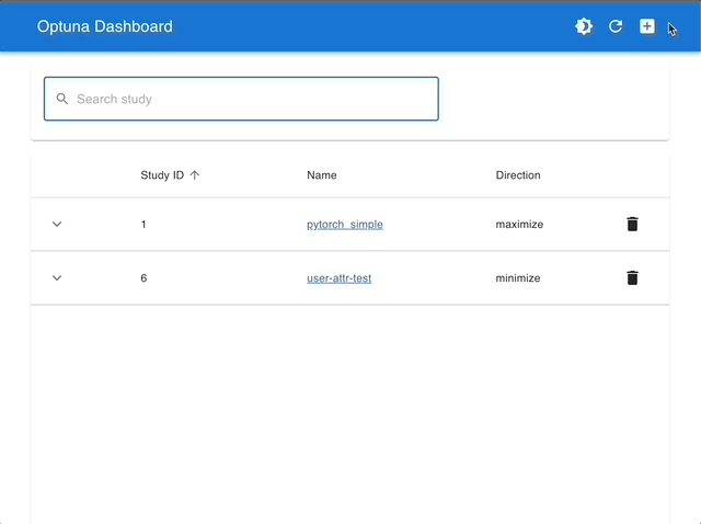
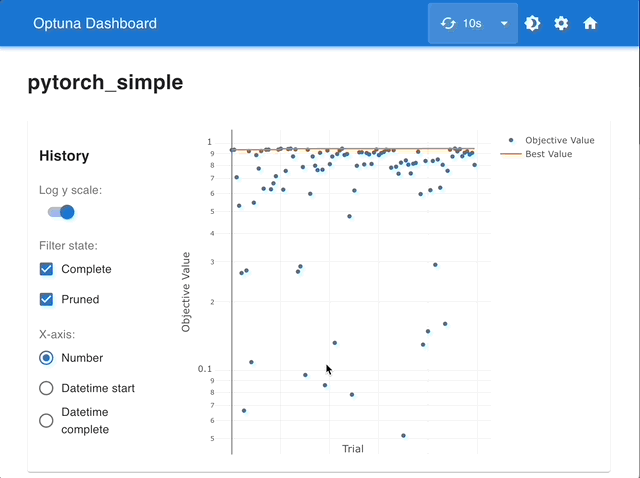
通过使用 Optuna Dashboard,您还可以在图表和表格中查看优化历史、超参数重要性、超参数关系等。请使用 RDB 后端 使您的研究持久化,并执行以下命令来运行 Optuna Dashboard。
$ pip install optuna-dashboard
$ optuna-dashboard sqlite:///example-study.db
更多详情请查看 GitHub 仓库。
管理研究 |
使用交互式图表进行可视化 |
|---|---|
|
|
import torch
import torch.nn as nn
import torch.nn.functional as F
import torchvision


import optuna

# You can use Matplotlib instead of Plotly for visualization by simply replacing `optuna.visualization` with
# `optuna.visualization.matplotlib` in the following examples.
from optuna.visualization import plot_contour
from optuna.visualization import plot_edf
from optuna.visualization import plot_intermediate_values
from optuna.visualization import plot_optimization_history
from optuna.visualization import plot_parallel_coordinate
from optuna.visualization import plot_param_importances
from optuna.visualization import plot_rank
from optuna.visualization import plot_slice
from optuna.visualization import plot_timeline


SEED = 13
torch.manual_seed(SEED)

DEVICE = torch.device("cuda") if torch.cuda.is_available() else torch.device("cpu")
DIR = ".."
BATCHSIZE = 128
N_TRAIN_EXAMPLES = BATCHSIZE * 30
N_VALID_EXAMPLES = BATCHSIZE * 10


def define_model(trial):
    n_layers = trial.suggest_int("n_layers", 1, 2)
    layers = []

    in_features = 28 * 28
    for i in range(n_layers):
        out_features = trial.suggest_int("n_units_l{}".format(i), 64, 512)
        layers.append(nn.Linear(in_features, out_features))
        layers.append(nn.ReLU())

        in_features = out_features

    layers.append(nn.Linear(in_features, 10))
    layers.append(nn.LogSoftmax(dim=1))

    return nn.Sequential(*layers)


# Defines training and evaluation.
def train_model(model, optimizer, train_loader):
    model.train()
    for batch_idx, (data, target) in enumerate(train_loader):
        data, target = data.view(-1, 28 * 28).to(DEVICE), target.to(DEVICE)
        optimizer.zero_grad()
        F.nll_loss(model(data), target).backward()
        optimizer.step()


def eval_model(model, valid_loader):
    model.eval()
    correct = 0
    with torch.no_grad():
        for batch_idx, (data, target) in enumerate(valid_loader):
            data, target = data.view(-1, 28 * 28).to(DEVICE), target.to(DEVICE)
            pred = model(data).argmax(dim=1, keepdim=True)
            correct += pred.eq(target.view_as(pred)).sum().item()

    accuracy = correct / N_VALID_EXAMPLES

    return accuracy
定义目标函数。
def objective(trial):
    train_dataset = torchvision.datasets.FashionMNIST(
        DIR, train=True, download=True, transform=torchvision.transforms.ToTensor()
    )
    train_loader = torch.utils.data.DataLoader(
        torch.utils.data.Subset(train_dataset, list(range(N_TRAIN_EXAMPLES))),
        batch_size=BATCHSIZE,
        shuffle=True,
    )

    val_dataset = torchvision.datasets.FashionMNIST(
        DIR, train=False, transform=torchvision.transforms.ToTensor()
    )
    val_loader = torch.utils.data.DataLoader(
        torch.utils.data.Subset(val_dataset, list(range(N_VALID_EXAMPLES))),
        batch_size=BATCHSIZE,
        shuffle=True,
    )
    model = define_model(trial).to(DEVICE)

    optimizer = torch.optim.Adam(
        model.parameters(), trial.suggest_float("lr", 1e-5, 1e-1, log=True)
    )

    for epoch in range(10):
        train_model(model, optimizer, train_loader)

        val_accuracy = eval_model(model, val_loader)
        trial.report(val_accuracy, epoch)

        if trial.should_prune():
            raise optuna.exceptions.TrialPruned()

    return val_accuracy
study = optuna.create_study(
    direction="maximize",
    sampler=optuna.samplers.TPESampler(seed=SEED),
    pruner=optuna.pruners.MedianPruner(),
)
study.optimize(objective, n_trials=30, timeout=300)
Downloading http://fashion-mnist.s3-website.eu-central-1.amazonaws.com/train-images-idx3-ubyte.gz
Downloading http://fashion-mnist.s3-website.eu-central-1.amazonaws.com/train-images-idx3-ubyte.gz to ../FashionMNIST/raw/train-images-idx3-ubyte.gz

  0%|          | 0/26421880 [00:00<?, ?it/s]
  0%|          | 32768/26421880 [00:00<02:46, 158857.56it/s]
  0%|          | 65536/26421880 [00:00<02:45, 159671.99it/s]
  0%|          | 131072/26421880 [00:00<01:52, 233638.31it/s]
  1%|          | 196608/26421880 [00:00<01:36, 272804.28it/s]
  1%|▏         | 360448/26421880 [00:00<00:46, 562518.46it/s]
  2%|▏         | 458752/26421880 [00:01<00:39, 657751.04it/s]
  3%|▎         | 753664/26421880 [00:01<00:22, 1137627.78it/s]
  5%|▍         | 1212416/26421880 [00:01<00:12, 1994694.27it/s]
  6%|▌         | 1572864/26421880 [00:01<00:12, 2060297.35it/s]
 10%|█         | 2752512/26421880 [00:01<00:05, 4323326.34it/s]
 13%|█▎        | 3309568/26421880 [00:01<00:05, 4565239.90it/s]
 24%|██▎       | 6225920/26421880 [00:01<00:02, 8785525.06it/s]
 36%|███▋      | 9601024/26421880 [00:02<00:01, 11727980.31it/s]
 46%|████▋     | 12222464/26421880 [00:02<00:00, 14290448.70it/s]
 54%|█████▍    | 14286848/26421880 [00:02<00:00, 15529525.09it/s]
 61%|██████▏   | 16220160/26421880 [00:02<00:00, 16276128.83it/s]
 68%|██████▊   | 17891328/26421880 [00:02<00:00, 13905583.64it/s]
 79%|███████▊  | 20774912/26421880 [00:02<00:00, 16436042.66it/s]
 87%|████████▋ | 23003136/26421880 [00:02<00:00, 12428357.95it/s]
 93%|█████████▎| 24444928/26421880 [00:03<00:00, 7847392.17it/s]
100%|██████████| 26421880/26421880 [00:03<00:00, 7772728.14it/s]
Extracting ../FashionMNIST/raw/train-images-idx3-ubyte.gz to ../FashionMNIST/raw

Downloading http://fashion-mnist.s3-website.eu-central-1.amazonaws.com/train-labels-idx1-ubyte.gz
Downloading http://fashion-mnist.s3-website.eu-central-1.amazonaws.com/train-labels-idx1-ubyte.gz to ../FashionMNIST/raw/train-labels-idx1-ubyte.gz

  0%|          | 0/29515 [00:00<?, ?it/s]
100%|██████████| 29515/29515 [00:00<00:00, 197327.02it/s]
100%|██████████| 29515/29515 [00:00<00:00, 196998.88it/s]
Extracting ../FashionMNIST/raw/train-labels-idx1-ubyte.gz to ../FashionMNIST/raw

Downloading http://fashion-mnist.s3-website.eu-central-1.amazonaws.com/t10k-images-idx3-ubyte.gz
Downloading http://fashion-mnist.s3-website.eu-central-1.amazonaws.com/t10k-images-idx3-ubyte.gz to ../FashionMNIST/raw/t10k-images-idx3-ubyte.gz

  0%|          | 0/4422102 [00:00<?, ?it/s]
  1%|          | 32768/4422102 [00:00<00:31, 139398.62it/s]
  1%|▏         | 65536/4422102 [00:00<00:28, 151516.00it/s]
  3%|▎         | 131072/4422102 [00:00<00:18, 228296.72it/s]
  5%|▌         | 229376/4422102 [00:00<00:12, 334087.21it/s]
 11%|█         | 491520/4422102 [00:01<00:05, 671460.59it/s]
 15%|█▍        | 655360/4422102 [00:01<00:04, 773333.71it/s]
 23%|██▎       | 1015808/4422102 [00:01<00:02, 1317311.64it/s]
 44%|████▎     | 1933312/4422102 [00:01<00:00, 2797135.19it/s]
 62%|██████▏   | 2752512/4422102 [00:01<00:00, 4006436.44it/s]
 73%|███████▎  | 3244032/4422102 [00:01<00:00, 3937559.00it/s]
100%|██████████| 4422102/4422102 [00:01<00:00, 2556449.61it/s]
Extracting ../FashionMNIST/raw/t10k-images-idx3-ubyte.gz to ../FashionMNIST/raw

Downloading http://fashion-mnist.s3-website.eu-central-1.amazonaws.com/t10k-labels-idx1-ubyte.gz
Downloading http://fashion-mnist.s3-website.eu-central-1.amazonaws.com/t10k-labels-idx1-ubyte.gz to ../FashionMNIST/raw/t10k-labels-idx1-ubyte.gz

  0%|          | 0/5148 [00:00<?, ?it/s]
100%|██████████| 5148/5148 [00:00<00:00, 13336798.64it/s]
Extracting ../FashionMNIST/raw/t10k-labels-idx1-ubyte.gz to ../FashionMNIST/raw
绘图函数
可视化优化历史。详情请参阅 plot_optimization_history()。
plot_optimization_history(study)
可视化试验的学习曲线。详情请参见 plot_intermediate_values()。
plot_intermediate_values(study)
可视化高维参数关系。详情请参见 plot_parallel_coordinate()。
plot_parallel_coordinate(study)
选择要可视化的参数。
plot_parallel_coordinate(study, params=["lr", "n_layers"])
可视化超参数关系。详情请参见 plot_contour()。
plot_contour(study)
选择要可视化的参数。
plot_contour(study, params=["lr", "n_layers"])
将单个超参数可视化为切片图。详情请参见 plot_slice()。
plot_slice(study)
选择要可视化的参数。
plot_slice(study, params=["lr", "n_layers"])
可视化参数重要性。详情请参见 plot_param_importances()。
plot_param_importances(study)
通过超参数重要性了解哪些超参数影响试验持续时间。
optuna.visualization.plot_param_importances(
    study, target=lambda t: t.duration.total_seconds(), target_name="duration"
)
可视化经验分布函数。详情请参见 plot_edf()。
plot_edf(study)
通过散点图可视化参数关系,并根据目标值进行着色。详情请参见 plot_rank()。
plot_rank(study)
可视化执行试验的优化时间线。详情请参见 plot_timeline()。
plot_timeline(study)
自定义生成的图形
在 optuna.visualization 和 optuna.visualization.matplotlib 中,一个函数返回一个可编辑的图形对象:plotly.graph_objects.Figure 或 matplotlib.axes.Axes,取决于模块。这允许用户使用可视化库的API根据他们的需求修改生成的图形。以下示例手动替换由基于Plotly的 plot_intermediate_values() 绘制的图形标题。
fig = plot_intermediate_values(study)

fig.update_layout(
    title="Hyperparameter optimization for FashionMNIST classification",
    xaxis_title="Epoch",
    yaxis_title="Validation Accuracy",
)
脚本总运行时间: (0 分钟 53.291 秒)