使用N-HiTS进行多变量分位数和长期预测

import warnings

warnings.filterwarnings("ignore")

import lightning.pytorch as pl
from lightning.pytorch.callbacks import EarlyStopping
import matplotlib.pyplot as plt
import numpy as np
import pandas as pd
import torch

from pytorch_forecasting import Baseline, NHiTS, TimeSeriesDataSet
from pytorch_forecasting.data import NaNLabelEncoder
from pytorch_forecasting.data.examples import generate_ar_data
from pytorch_forecasting.metrics import MAE, SMAPE, MQF2DistributionLoss, QuantileLoss

加载数据

我们生成了一个合成数据集来展示网络的能力。数据包括一个二次趋势和一个季节性成分。

data = generate_ar_data(seasonality=10.0, timesteps=400, n_series=100, seed=42)
data["static"] = 2
data["date"] = pd.Timestamp("2020-01-01") + pd.to_timedelta(data.time_idx, "D")
data.head()

	系列	时间索引	值	静态	日期
0	0	0	-0.000000	2	2020-01-01
1	0	1	-0.046501	2	2020-01-02
2	0	2	-0.097796	2	2020-01-03
3	0	3	-0.144397	2	2020-01-04
4	0	4	-0.177954	2	2020-01-05

在开始训练之前，我们需要将数据集分割成训练和验证的TimeSeriesDataSet。

# create dataset and dataloaders
max_encoder_length = 60
max_prediction_length = 20

training_cutoff = data["time_idx"].max() - max_prediction_length

context_length = max_encoder_length
prediction_length = max_prediction_length

training = TimeSeriesDataSet(
    data[lambda x: x.time_idx <= training_cutoff],
    time_idx="time_idx",
    target="value",
    categorical_encoders={"series": NaNLabelEncoder().fit(data.series)},
    group_ids=["series"],
    # only unknown variable is "value" - and N-HiTS can also not take any additional variables
    time_varying_unknown_reals=["value"],
    max_encoder_length=context_length,
    max_prediction_length=prediction_length,
)

validation = TimeSeriesDataSet.from_dataset(training, data, min_prediction_idx=training_cutoff + 1)
batch_size = 128
train_dataloader = training.to_dataloader(train=True, batch_size=batch_size, num_workers=0)
val_dataloader = validation.to_dataloader(train=False, batch_size=batch_size, num_workers=0)

计算基线误差

我们的基线模型通过重复最后一个已知值来预测未来值。结果得到的SMAPE令人失望，应该不容易被超越。

# calculate baseline absolute error
baseline_predictions = Baseline().predict(val_dataloader, trainer_kwargs=dict(accelerator="cpu"), return_y=True)
SMAPE()(baseline_predictions.output, baseline_predictions.y)

GPU available: True (mps), used: False
TPU available: False, using: 0 TPU cores
IPU available: False, using: 0 IPUs
HPU available: False, using: 0 HPUs

tensor(0.5462)

训练网络

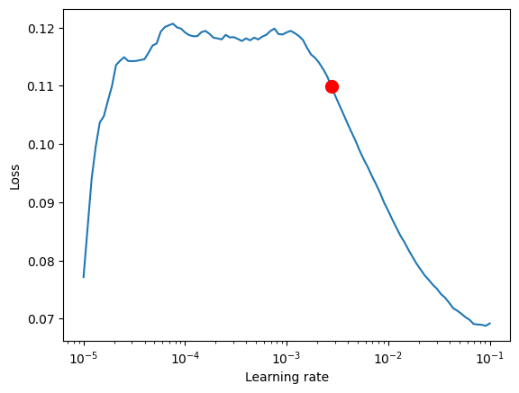
使用[PyTorch Lightning](https://pytorch-lightning.readthedocs.io/)找到最佳学习率很容易。NHiTS模型的关键超参数是hidden_size。

PyTorch Forecasting 足够灵活，可以使用 NHiTS 与不同的损失函数，不仅支持点预测，还支持概率预测。在这里，我们不仅将演示典型的分位数回归，还将演示使用 MQF2DistributionLoss 的多变量分位数回归，该回归允许沿预测范围计算采样一致的路径。这使得可以计算分位数，例如预测范围内的总和，同时仍然避免像 DeepAR 这样的自回归方法中的累积误差问题。为此，需要安装一个额外的包来实现此分位数函数：

pip install pytorch-forecasting[mqf2]

pl.seed_everything(42)
trainer = pl.Trainer(accelerator="cpu", gradient_clip_val=0.1)
net = NHiTS.from_dataset(
    training,
    learning_rate=3e-2,
    weight_decay=1e-2,
    loss=MQF2DistributionLoss(prediction_length=max_prediction_length),
    backcast_loss_ratio=0.0,
    hidden_size=64,
    optimizer="AdamW",
)

Global seed set to 42
GPU available: True (mps), used: False
TPU available: False, using: 0 TPU cores
IPU available: False, using: 0 IPUs
HPU available: False, using: 0 HPUs

# find optimal learning rate
from lightning.pytorch.tuner import Tuner

res = Tuner(trainer).lr_find(
    net, train_dataloaders=train_dataloader, val_dataloaders=val_dataloader, min_lr=1e-5, max_lr=1e-1
)
print(f"suggested learning rate: {res.suggestion()}")
fig = res.plot(show=True, suggest=True)
fig.show()
net.hparams.learning_rate = res.suggestion()

`Trainer.fit` stopped: `max_steps=100` reached.
Learning rate set to 0.0027542287033381664
Restoring states from the checkpoint path at /Users/JanBeitner/Documents/code/pytorch-forecasting/.lr_find_9ea79aec-8577-4e17-859e-f46d818dbf70.ckpt
Restored all states from the checkpoint at /Users/JanBeitner/Documents/code/pytorch-forecasting/.lr_find_9ea79aec-8577-4e17-859e-f46d818dbf70.ckpt

suggested learning rate: 0.0027542287033381664

拟合模型

early_stop_callback = EarlyStopping(monitor="val_loss", min_delta=1e-4, patience=10, verbose=False, mode="min")
trainer = pl.Trainer(
    max_epochs=5,
    accelerator="cpu",
    enable_model_summary=True,
    gradient_clip_val=1.0,
    callbacks=[early_stop_callback],
    limit_train_batches=30,
    enable_checkpointing=True,
)


net = NHiTS.from_dataset(
    training,
    learning_rate=5e-3,
    log_interval=10,
    log_val_interval=1,
    weight_decay=1e-2,
    backcast_loss_ratio=0.0,
    hidden_size=64,
    optimizer="AdamW",
    loss=MQF2DistributionLoss(prediction_length=max_prediction_length),
)

trainer.fit(
    net,
    train_dataloaders=train_dataloader,
    val_dataloaders=val_dataloader,
)

GPU available: True (mps), used: False
TPU available: False, using: 0 TPU cores
IPU available: False, using: 0 IPUs
HPU available: False, using: 0 HPUs

  | Name            | Type                 | Params
---------------------------------------------------------
0 | loss            | MQF2DistributionLoss | 5.1 K
1 | logging_metrics | ModuleList           | 0
2 | embeddings      | MultiEmbedding       | 0
3 | model           | NHiTS                | 35.7 K
---------------------------------------------------------
40.8 K    Trainable params
0         Non-trainable params
40.8 K    Total params
0.163     Total estimated model params size (MB)

`Trainer.fit` stopped: `max_epochs=5` reached.

评估结果

best_model_path = trainer.checkpoint_callback.best_model_path
best_model = NHiTS.load_from_checkpoint(best_model_path)

我们在验证数据集上使用predict()进行预测，并计算误差，该误差远低于基线误差

predictions = best_model.predict(val_dataloader, trainer_kwargs=dict(accelerator="cpu"), return_y=True)
MAE()(predictions.output, predictions.y)

GPU available: True (mps), used: False
TPU available: False, using: 0 TPU cores
IPU available: False, using: 0 IPUs
HPU available: False, using: 0 HPUs

tensor(0.2012)

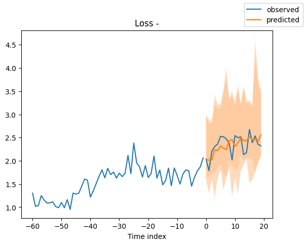
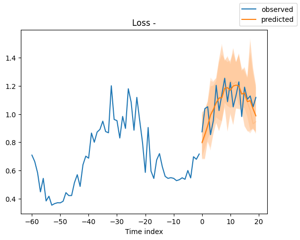
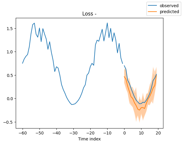
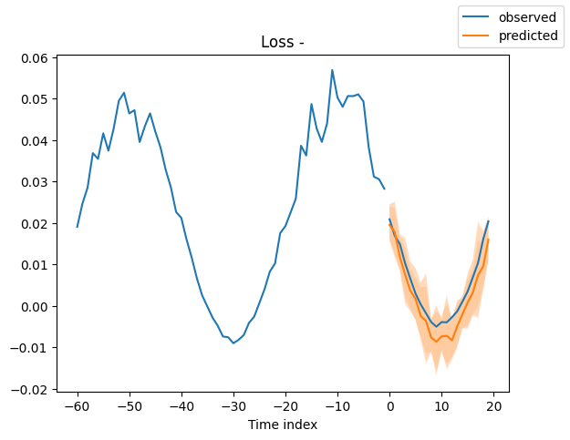
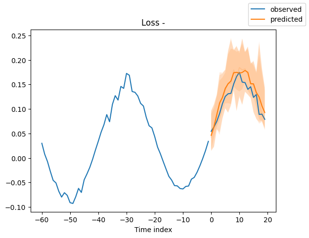
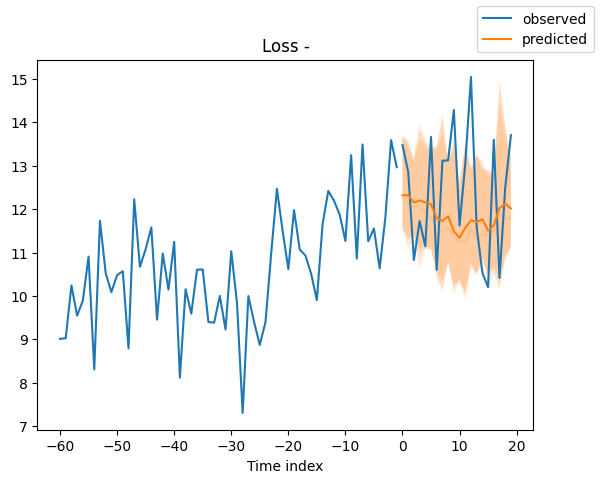
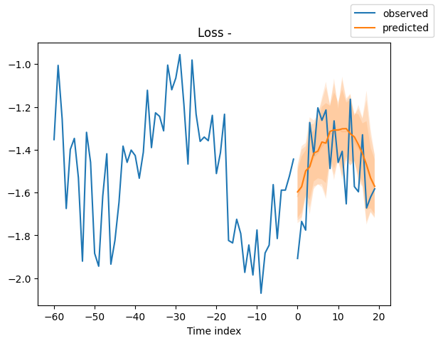
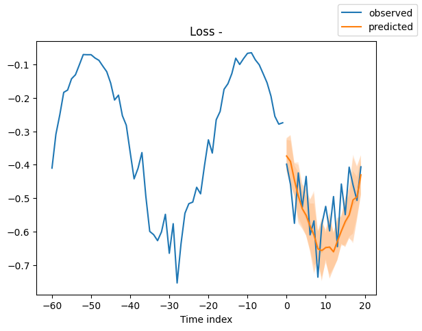
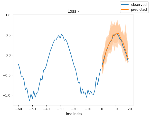
查看验证集中的随机样本总是了解预测是否合理的好方法 - 确实如此！

raw_predictions = best_model.predict(val_dataloader, mode="raw", return_x=True, trainer_kwargs=dict(accelerator="cpu"))

GPU available: True (mps), used: False
TPU available: False, using: 0 TPU cores
IPU available: False, using: 0 IPUs
HPU available: False, using: 0 HPUs

for idx in range(10):  # plot 10 examples
    best_model.plot_prediction(raw_predictions.x, raw_predictions.output, idx=idx, add_loss_to_title=True)

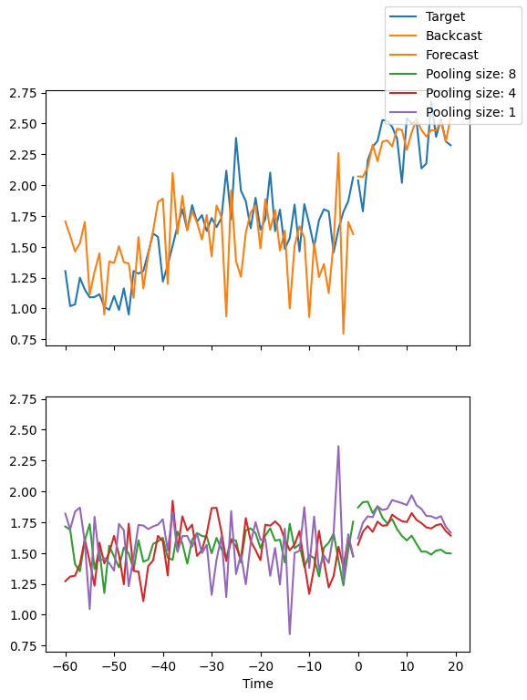
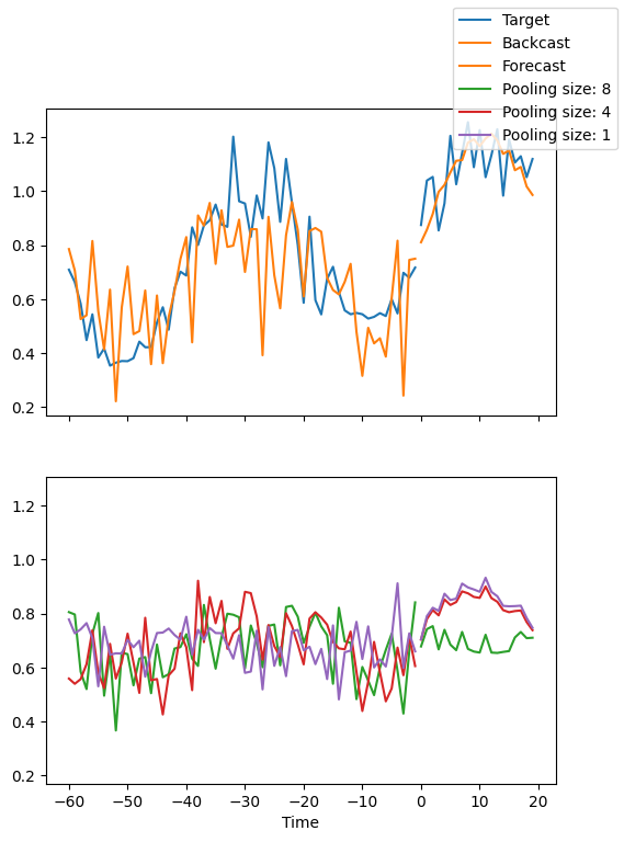
解释模型

我们可以要求PyTorch Forecasting将预测分解为专注于不同频谱的块，例如使用plot_interpretation()的季节性和趋势。这是NHiTS模型的一个特殊功能，只有其独特的架构才能实现。结果显示，似乎有很多方法可以解释数据，而算法并不总是选择直观上有意义的方法。这部分是因为我们训练的时间序列数量较少（100个）。但这也是因为我们的预测期没有涵盖多个季节性。

for idx in range(2):  # plot 10 examples
    best_model.plot_interpretation(raw_predictions.x, raw_predictions.output, idx=idx)

从预测中采样

# sample 500 paths
samples = best_model.loss.sample(raw_predictions.output["prediction"][[0]], n_samples=500)[0]

# plot prediction
fig = best_model.plot_prediction(raw_predictions.x, raw_predictions.output, idx=0, add_loss_to_title=True)
ax = fig.get_axes()[0]
# plot first two sampled paths
ax.plot(samples[:, 0], color="g", label="Sample 1")
ax.plot(samples[:, 1], color="r", label="Sample 2")
fig.legend()

<matplotlib.legend.Legend at 0x2dea42680>

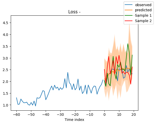
正如预期的那样，每个样本内的预测方差比所有样本之间的方差要小。

print(f"Var(all samples) = {samples.var():.4f}")
print(f"Mean(Var(sample)) = {samples.var(0).mean():.4f}")

Var(all samples) = 0.2084
Mean(Var(sample)) = 0.1616

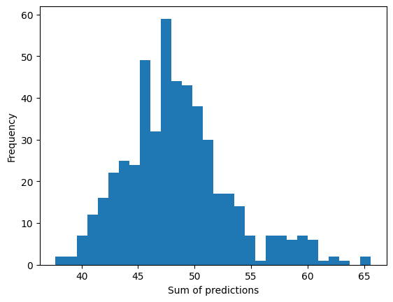
我们现在可以做些新的事情，并绘制整个预测范围内预测总和的分布。

plt.hist(samples.sum(0).numpy(), bins=30)
plt.xlabel("Sum of predictions")
plt.ylabel("Frequency")

Text(0, 0.5, 'Frequency')