statsmodels.graphics.gofplots.ProbPlot¶

class statsmodels.graphics.gofplots.ProbPlot(data, dist=<scipy.stats._continuous_distns.norm_gen object>, fit=False, distargs=(), a=0, loc=0, scale=1)[source]¶

Q-Q 和 P-P 概率图

可以接受指定分布参数的参数，或自动拟合这些参数。（参见 kwargs 下的 fit。）

Parameters:¶

dataarray_like

一维数据数组

distcallable

将x与dist进行比较。dist可以是scipy.stats或statsmodels分布。默认值为scipy.stats.distributions.norm（标准正态分布）。可以是SciPy冻结分布。

fitbool

如果 fit 为 false，loc、scale 和 distargs 将被传递给分布。如果 fit 为 True，则使用 dist.fit 自动拟合 dist 的参数。分位数是通过标准化数据形成的，在减去拟合的 loc 并除以拟合的 scale 之后。如果 dist 是 SciPy 冻结分布，则不能使用 fit。

distargstuple

传递给 dist 的参数元组，以完全指定它，从而可以调用 dist.ppf。distargs 不得包含 loc 或 scale。这些值必须使用 loc 或 scale 输入来传递。如果 dist 是 SciPy 冻结分布，则不能使用 distargs。

afloat

用于预期顺序统计量的绘图位置的偏移量，例如。绘图位置由 (i - a)/(nobs - 2*a + 1) 给出，其中 i 在 range(0, nobs+1) 范围内

locfloat

分布的位置参数。如果dist是SciPy冻结分布，则不能使用。

scalefloat

dist 的比例参数。如果 dist 是 SciPy 冻结分布，则不能使用。

Attributes:¶

sample_percentiles

样本百分位数

sample_quantiles

样本分位数

sorted_data

排序后的数据

theoretical_percentiles

理论百分位数

theoretical_quantiles

理论分位数

另请参阅

scipy.stats.probplot

注释

1. 依赖于matplotlib。

2. If fit is True then the parameters are fit using the

   分布的 fit() 方法。

3. The call signatures for the qqplot, ppplot, and probplot

   方法类似，因此示例1到4适用于所有三种方法。

4. The three plotting methods are summarized below:

   ppplotProbability-Probability plot

   比较样本和理论概率（百分位数）。

   qqplotQuantile-Quantile plot

   比较样本和理论分位数

   probplotProbability plot

   与Q-Q图相同，但概率以理论分布的尺度（x轴）显示，y轴包含样本数据的未缩放分位数。

示例

第一个示例展示了回归残差的Q-Q图

>>> # example 1
>>> import statsmodels.api as sm
>>> from matplotlib import pyplot as plt
>>> data = sm.datasets.longley.load()
>>> data.exog = sm.add_constant(data.exog)
>>> model = sm.OLS(data.endog, data.exog)
>>> mod_fit = model.fit()
>>> res = mod_fit.resid # residuals
>>> pplot = sm.ProbPlot(res)
>>> fig = pplot.qqplot()
>>> h = plt.title("Ex. 1 - qqplot - residuals of OLS fit")
>>> plt.show()

残差与自由度为4的t分布分位数的qq图：

>>> # example 2
>>> import scipy.stats as stats
>>> pplot = sm.ProbPlot(res, stats.t, distargs=(4,))
>>> fig = pplot.qqplot()
>>> h = plt.title("Ex. 2 - qqplot - residuals against quantiles of t-dist")
>>> plt.show()

qq图与上述相同，但均值为3，标准差为10：

>>> # example 3
>>> pplot = sm.ProbPlot(res, stats.t, distargs=(4,), loc=3, scale=10)
>>> fig = pplot.qqplot()
>>> h = plt.title("Ex. 3 - qqplot - resids vs quantiles of t-dist")
>>> plt.show()

自动确定t分布的参数，包括loc和scale：

>>> # example 4
>>> pplot = sm.ProbPlot(res, stats.t, fit=True)
>>> fig = pplot.qqplot(line="45")
>>> h = plt.title("Ex. 4 - qqplot - resids vs. quantiles of fitted t-dist")
>>> plt.show()

第二个 ProbPlot 对象可以用于通过在 qqplot 和 ppplot 方法中使用 other kwarg 来比较两个独立的样本集。

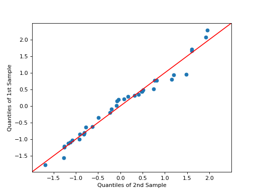
>>> # example 5
>>> import numpy as np
>>> x = np.random.normal(loc=8.25, scale=2.75, size=37)
>>> y = np.random.normal(loc=8.75, scale=3.25, size=37)
>>> pp_x = sm.ProbPlot(x, fit=True)
>>> pp_y = sm.ProbPlot(y, fit=True)
>>> fig = pp_x.qqplot(line="45", other=pp_y)
>>> h = plt.title("Ex. 5 - qqplot - compare two sample sets")
>>> plt.show()

在qqplot中，other的样本大小可以等于或大于第一个。如果大于，other样本的大小将通过插值减少以匹配第一个样本的大小。

>>> # example 6
>>> x = np.random.normal(loc=8.25, scale=2.75, size=37)
>>> y = np.random.normal(loc=8.75, scale=3.25, size=57)
>>> pp_x = sm.ProbPlot(x, fit=True)
>>> pp_y = sm.ProbPlot(y, fit=True)
>>> fig = pp_x.qqplot(line="45", other=pp_y)
>>> title = "Ex. 6 - qqplot - compare different sample sizes"
>>> h = plt.title(title)
>>> plt.show()

在ppplot中，other的样本大小和第一个可以不同。other 将用于估计经验累积分布函数（ECDF）。ECDF(x)将与p(x)=0.5/n, 1.5/n, …, (n-0.5)/n 进行绘图，其中x是从第一个排序后的样本。

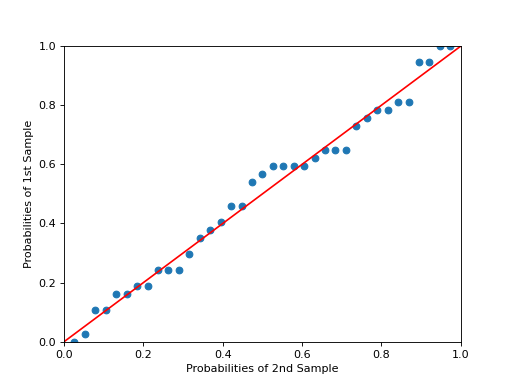
>>> # example 7
>>> x = np.random.normal(loc=8.25, scale=2.75, size=37)
>>> y = np.random.normal(loc=8.75, scale=3.25, size=57)
>>> pp_x = sm.ProbPlot(x, fit=True)
>>> pp_y = sm.ProbPlot(y, fit=True)
>>> pp_y.ppplot(line="45", other=pp_x)
>>> plt.title("Ex. 7A- ppplot - compare two sample sets, other=pp_x")
>>> pp_x.ppplot(line="45", other=pp_y)
>>> plt.title("Ex. 7B- ppplot - compare two sample sets, other=pp_y")
>>> plt.show()

以下图表展示了一些选项，请点击链接查看代码。

(源代码)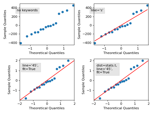

方法

ppplot([xlabel, ylabel, line, other, ax])	x的百分位数与分布的百分位数的图表。
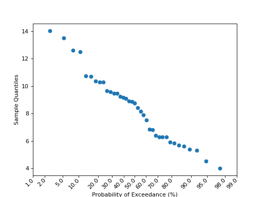
probplot([xlabel, ylabel, line, exceed, ax])	未缩放的分位数x与分布概率的图。
qqplot([xlabel, ylabel, line, other, ax, swap])	x的分位数与分布的分位数/ppf的对比图。

属性

sample_percentiles	样本百分位数
sample_quantiles	样本分位数
sorted_data	排序后的数据
theoretical_percentiles	理论百分位数
theoretical_quantiles	理论分位数