statsmodels.tsa.filters.bk_filter.bkfilter
-
statsmodels.tsa.filters.bk_filter.bkfilter(x, low=
6, high=32, K=12)[source]¶ 使用Baxter-King带通滤波器过滤时间序列。
- Parameters:
- xarray_like
一个1维或2维的ndarray。如果是2维的,变量假设在列中。
- low
float 振荡的最小周期,即Baxter和King建议,Burns-Mitchell美国经济周期对于季度数据为6,对于年度数据为1.5。
- high
float BK建议的最大周期表明,美国商业周期对于季度数据为32,对于年度数据为8。
- K
int 滤波器的领先滞后长度。Baxter和King建议对于季度数据截断长度为12,对于年度数据截断长度为3。
- Returns:
ndarrayx的周期性成分。
另请参阅
statsmodels.tsa.filters.cf_filter.cffilterChristiano Fitzgerald 非对称随机游走滤波器。
statsmodels.tsa.filters.bk_filter.hpfilterHodrick-Prescott 滤波器。
statsmodels.tsa.seasonal.seasonal_decompose使用移动平均法分解时间序列。
statsmodels.tsa.seasonal.STL使用LOESS进行季节趋势分解。
注释
返回原始序列的居中加权移动平均值。其中权重 a[j] 是计算得出的
a[j] = b[j] + theta, for j = 0, +/-1, +/-2, ... +/- K
b[0] = (omega_2 - omega_1)/pi
b[j] = 1/(pi*j)(sin(omega_2*j)-sin(omega_1*j), for j = +/-1, +/-2,...
并且 theta 是一个归一化常数
theta = -sum(b)/(2K+1)请参阅笔记本 时间序列过滤器 以获取概述。
参考文献
- Baxter, M. and R. G. King. “Measuring Business Cycles: Approximate
带通滤波器用于经济时间序列。” 经济学与统计学评论,1999年,81(4),575-593。
示例
>>> import statsmodels.api as sm
>>> import pandas as pd
>>> dta = sm.datasets.macrodata.load_pandas().data
>>> index = pd.DatetimeIndex(start='1959Q1', end='2009Q4', freq='Q')
>>> dta.set_index(index, inplace=True)
>>> cycles = sm.tsa.filters.bkfilter(dta[['realinv']], 6, 24, 12)>>> import matplotlib.pyplot as plt >>> fig, ax = plt.subplots() >>> cycles.plot(ax=ax, style=['r--', 'b-']) >>> plt.show()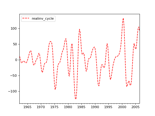
Last update:
Oct 16, 2024