使用QAT微调Llama3
量化感知训练(QAT)是一种常见的技术,用户可以通过它量化他们的模型,而不会导致准确性或困惑度的显著下降。在本教程中,我们将逐步介绍如何在微调过程中应用QAT,量化生成的模型,并使用torchtune评估您的量化模型。
什么是QAT以及它如何帮助减少量化退化
如何在torchtune的微调过程中运行QAT
连接QAT、量化和评估配方的端到端示例
熟悉 torchtune
请确保您已下载Llama3-8B模型权重
什么是QAT?
Quantization-Aware Training (QAT) 指的是在训练或微调过程中模拟量化数值,最终目标是相比简单的训练后量化(PTQ)产生更高质量的量化模型。在QAT过程中,权重和/或激活被“伪量化”,这意味着它们被转换得好像被量化了一样,但仍保持在原始数据类型(例如bfloat16)中,而实际上并未被转换为更低的位宽。因此,伪量化允许模型在更新权重时调整量化噪声,因此训练过程“知道”模型最终将在训练后被量化。
# PTQ: x_q is quantized and cast to int8
# scale and zero point (zp) refer to parameters used to quantize x_float
# qmin and qmax refer to the range of quantized values
x_q = (x_float / scale + zp).round().clamp(qmin, qmax).cast(int8)

# QAT: x_fq is still in float
# Fake quantize simulates the numerics of quantize + dequantize
x_fq = (x_float / scale + zp).round().clamp(qmin, qmax)
x_fq = (x_fq - zp) * scale
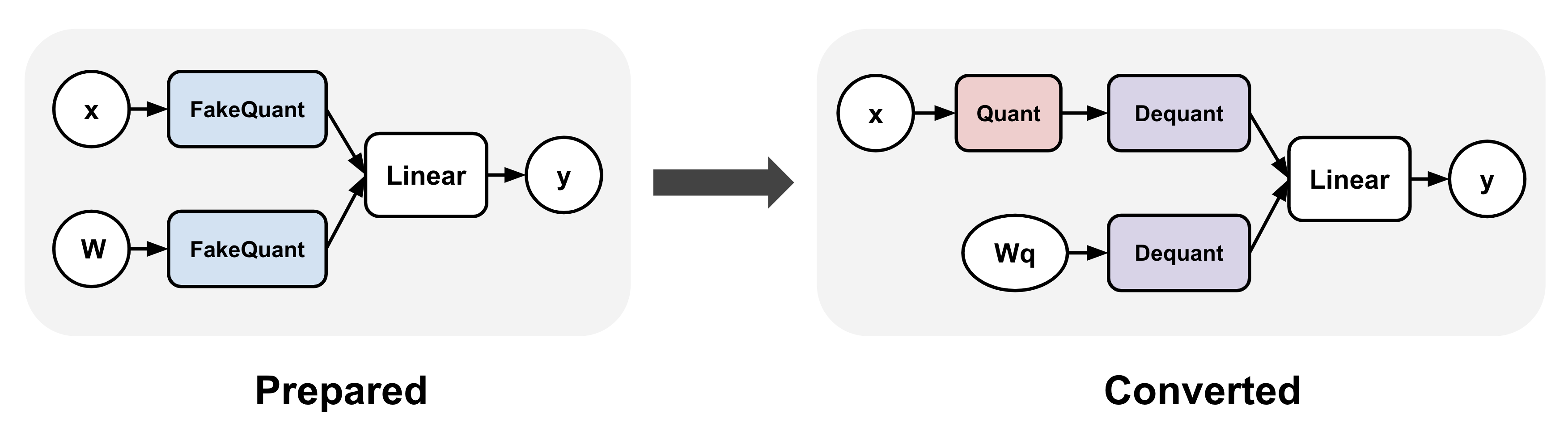
QAT通常涉及在训练前后对模型应用转换。
例如,在torchao QAT实现中,
这些步骤表示为prepare()和convert()步骤:(1) prepare()将伪量化操作插入到线性层中,(2) convert()在训练后将伪量化操作转换为实际的量化和反量化操作,从而生成量化模型(反量化操作通常在降低后与线性层融合)。
在这两个步骤之间,训练可以像以前一样进行。
将QAT应用于Llama3模型
我们可以轻松地将上述QAT转换应用于torchtune中的Llama3进行微调:
from torchtune.training.quantization import Int8DynActInt4WeightQATQuantizer
from torchtune.models.llama3 import llama3_8b

model = llama3_8b()

# Quantizer for int8 dynamic per token activations +
# int4 grouped per channel weights, only for linear layers
quantizer = Int8DynActInt4WeightQATQuantizer()

# Insert "fake quantize" operations into linear layers.
# These operations simulate quantization numerics during
# fine-tuning without performing any dtype casting
prepared_model = quantizer.prepare(model)
如果我们打印模型,我们会看到所有的线性层都已被替换为
Int8DynActInt4WeightQATLinear,它模拟了每令牌动态激活的int8数值 + 每通道分组的int4权重。现在模型已经准备好进行微调了。
>>> print(model.layers[0].attn)
MultiHeadAttention(
  (q_proj): Linear(in_features=4096, out_features=4096, bias=False)
  (k_proj): Linear(in_features=4096, out_features=1024, bias=False)
  (v_proj): Linear(in_features=4096, out_features=1024, bias=False)
  (output_proj): Linear(in_features=4096, out_features=4096, bias=False)
  (pos_embeddings): RotaryPositionalEmbeddings()
)

>>> print(prepared_model.layers[0].attn)
MultiHeadAttention(
  (q_proj): Int8DynActInt4WeightQATLinear(in_features=4096, out_features=4096, bias=False)
  (k_proj): Int8DynActInt4WeightQATLinear(in_features=4096, out_features=1024, bias=False)
  (v_proj): Int8DynActInt4WeightQATLinear(in_features=4096, out_features=1024, bias=False)
  (output_proj): Int8DynActInt4WeightQATLinear(in_features=4096, out_features=4096, bias=False)
  (pos_embeddings): RotaryPositionalEmbeddings()
)
微调后,我们可以转换模型以获得实际的量化模型。 如果我们打印转换后的模型,我们会看到QAT线性层已被替换为Int8DynActInt4WeightLinear,这是线性层的量化版本。 然后可以将此量化模型保存到检查点并用于推理或生成。
# Fine-tune as before
train_loop(prepared_model)

# Convert fake quantize to actual quantize operations
converted_model = quantizer.convert(prepared_model)
>>> print(converted_model.layers[0].attn)
MultiHeadAttention(
  (q_proj): Int8DynActInt4WeightLinear()
  (k_proj): Int8DynActInt4WeightLinear()
  (v_proj): Int8DynActInt4WeightLinear()
  (output_proj): Int8DynActInt4WeightLinear()
  (pos_embeddings): RotaryPositionalEmbeddings()
)
torchtune中的QAT微调配方
将所有内容整合在一起,我们现在可以使用torchtune的QAT配方来微调模型。 请确保您已经按照这些说明下载了Llama3的权重和分词器。在本教程中, 我们使用以下设置来展示QAT在恢复量化退化方面的有效性,与直接量化未使用QAT微调的模型相比。 您可以复制默认的QAT配置并进行以下相应的修改:
tune cp llama3/8B_qat_full custom_8B_qat_full.yaml
# Dataset
dataset:
  _component_: torchtune.datasets.text_completion_dataset
  source: allenai/c4
  max_seq_len: 8192
  column: text
  name: en
  split: train
seed: null
shuffle: True

...

epochs: 1
max_steps_per_epoch: 2000
fake_quant_after_n_steps: 1000
memory_efficient_fsdp_wrap: False
根据经验,我们观察到在前N步禁用伪量化会带来更好的结果,可能是因为这样做可以在我们开始向微调过程引入量化噪声之前让权重稳定下来。因此,这里我们在前1000步禁用伪量化。
然后,您可以使用以下命令通过上述配置运行QAT微调。此工作负载至少需要6个GPU,每个GPU的VRAM至少为80GB。默认情况下,此配置使用如上所示的int8动态每令牌激活 + int4每通道分组权重量化配置:
tune run --nnodes 1 --nproc_per_node 6 qat_distributed --config custom_8B_qat_full.yaml
注意
确保指向您的Llama3权重和分词器的位置。这可以通过添加checkpointer.checkpoint_files=[my_model_checkpoint_path] tokenizer_checkpoint=my_tokenizer_checkpoint_path
或直接修改8B_qat_full.yaml文件来完成。有关如何轻松克隆和修改torchtune配置的更多详细信息,请参阅我们的关于配置的一切。
注意
与常规微调相比,QAT引入了内存和计算开销,因为伪量化本质上涉及额外的操作,并且需要克隆权重以避免在计算伪量化值时改变它们。一般来说,我们预计像Llama3-8B这样的模型的微调速度会降低约30%。使用激活检查点时,每个GPU的内存占用增加是最小的(每个GPU小于5GB)。
量化QAT模型
请注意,上述QAT配方生成的是一个未量化的bfloat16模型。该模型结构与不使用QAT的常规全微调生成的模型完全相同,只是权重不同。要实际获得量化模型,请复制并对量化配置进行以下修改:
tune cp quantization custom_quantization.yaml
# Model arguments
model:
  _component_: torchtune.models.llama3.llama3_8b

checkpointer:
  _component_: torchtune.training.FullModelMetaCheckpointer
  checkpoint_dir: <your QAT checkpoint dir>
  checkpoint_files: [meta_model_0.pt]
  recipe_checkpoint: null
  output_dir: <your QAT checkpoint dir>
  model_type: LLAMA3

...

quantizer:
  _component_: torchtune.training.quantization.Int8DynActInt4WeightQATQuantizer
  groupsize: 256
以下命令执行QAT流程中的转换步骤,实际上将浮点模型量化为具有量化权重的模型:
tune run quantize --config custom_quantization.yaml
注意
确保使用与微调模型时相同的QAT量化器,否则数值将不准确,量化模型的性能将较差。
评估量化模型
现在我们有了一个量化模型,我们可以对其进行一些评估,并将结果与没有QAT(即训练后量化)的常规微调进行比较。为此,我们使用EleutherAI的评估工具,该工具已集成到torchtune中。首先,复制评估配置并进行以下更改:
tune cp eleuther_evaluation custom_eleuther_evaluation.yaml
# Model arguments
model:
  _component_: torchtune.models.llama3.llama3_8b

checkpointer:
  _component_: torchtune.training.FullModelTorchTuneCheckpointer
  checkpoint_dir: <your quantized model checkpoint dir>
  checkpoint_files: [meta_model_0-8da4w.pt]
  recipe_checkpoint: null
  output_dir: <your quantized model checkpoint dir>
  model_type: LLAMA3

...

# EleutherAI specific eval args
tasks: ["hellaswag", "wikitext"]
limit: null
max_seq_length: 8192
batch_size: 8

quantizer:
  _component_: torchtune.training.quantization.Int8DynActInt4WeightQuantizer
  groupsize: 256
注意
由于我们传入的是量化模型,请确保使用相应的训练后量化器而不是QAT量化器。例如,如果在微调期间使用了Int8DynActInt4WeightQATQuantizer,您应该在此步骤中指定Int8DynActInt4WeightQuantizer。请参阅量化配方以获取支持的量化器的完整列表。
现在运行评估配方:
tune run eleuther_eval --config my_eleuther_evaluation.yaml
结果应该看起来像这样:
# QAT quantized model evaluation results (int8 activations + int4 weights)

|  Tasks  |Version|Filter|n-shot|    Metric     |Value |   |Stderr|
|---------|------:|------|-----:|---------------|-----:|---|------|
|wikitext |      2|none  |     0|word_perplexity|9.9148|±  |N/A   |
|         |       |none  |     0|byte_perplexity|1.5357|±  |N/A   |
|         |       |none  |     0|bits_per_byte  |0.6189|±  |N/A   |
|hellaswag|      1|none  |     0|acc            |0.5687|±  |0.0049|
|         |       |none  |     0|acc_norm       |0.7536|±  |0.0043|
将这些结果与未使用QAT进行微调的模型进行比较,我们可以看到,与PTQ相比,QAT能够从原始未量化模型中恢复量化退化的显著部分。例如,在hellaswag任务中,与原始未量化模型相比,PTQ的归一化准确率下降了2.20%,而QAT仅下降了0.74%。同样,在wikitext任务中,PTQ的单词困惑度增加了2.048,而QAT仅增加了1.190(越低越好)。
# PTQ quantized model evaluation results (int8 activations + int4 weights)

|  Tasks  |Version|Filter|n-shot|    Metric     | Value |   |Stderr|
|---------|------:|------|-----:|---------------|------:|---|------|
|wikitext |      2|none  |     0|word_perplexity|10.7735|±  |N/A   |
|         |       |none  |     0|byte_perplexity| 1.5598|±  |N/A   |
|         |       |none  |     0|bits_per_byte  | 0.6413|±  |N/A   |
|hellaswag|      1|none  |     0|acc            | 0.5481|±  |0.0050|
|         |       |none  |     0|acc_norm       | 0.7390|±  |0.0044|
# Float model evaluation results (bfloat16)

|  Tasks  |Version|Filter|n-shot|    Metric     |Value |   |Stderr|
|---------|------:|------|-----:|---------------|-----:|---|------|
|wikitext |      2|none  |     0|word_perplexity|8.7251|±  |N/A   |
|         |       |none  |     0|byte_perplexity|1.4994|±  |N/A   |
|         |       |none  |     0|bits_per_byte  |0.5844|±  |N/A   |
|hellaswag|      1|none  |     0|acc            |0.5740|±  |0.0049|
|         |       |none  |     0|acc_norm       |0.7610|±  |0.0043|
因此,QAT流程生成的量化模型优于训练后量化模型。重要的是,量化模型的结构在两种流程中是相同的,因此模型大小、内存使用量以及所有其他性能特征也相同。
请注意,尽管权重被量化为int4,但QAT和PTQ流程的量化模型大小均为8.187 GB,而原始浮点模型为14.958 GB。这是因为该量化器使用int8来表示权重,因为PyTorch没有原生的int4数据类型支持。更有效的表示方法是打包int4权重,这将使量化模型大小减半。这就是Int4WeightOnlyQuantizer所做的,相应的QAT量化器将在未来添加。
将QAT模型部署到设备(可选)
量化模型的一个重要动机是能够在资源受限的环境中运行它。你可以通过遵循这些说明,使用executorch进一步将你的QAT Llama3模型降低到智能手机等边缘设备。例如,以下命令将模型降低到XNNPACK后端:
python -m examples.models.llama2.export_llama --checkpoint <your QAT checkpoint> -p <params.json> -kv --use_sdpa_with_kv_cache -X -qmode 8da4w --group_size 256 -d fp32 --metadata '{"get_bos_id":128000, "get_eos_id":128001}' --embedding-quantize 4,32 --output_name="llama3_8da4w.pte"
这导致了一个更小的量化模型,大小为3.881 GB。在OnePlus 12智能手机上进行基准测试时,该模型也达到了与训练后量化模型相同的推理和生成速度。这是因为两种流程中的模型结构是相同的:
QAT |
PTQ |
|
|---|---|---|
量化模型大小 |
3.881 GB |
3.881 GB |
推理速度 |
9.709 令牌/秒 |
9.815 令牌/秒 |
生成速度 |
11.316 令牌/秒 |
11.364 令牌/秒 |
