使用torchaudio进行音频处理

torchaudio 提供了强大的音频输入输出功能、预处理转换和数据集。

在本教程中，我们将探讨如何准备音频数据并提取可以输入到神经网络模型中的特征。

# When running this tutorial in Google Colab, install the required packages
# with the following.
# !pip install torchaudio librosa boto3

import torch
import torchaudio
import torchaudio.functional as F
import torchaudio.transforms as T

print(torch.__version__)
print(torchaudio.__version__)

输出:

1.10.0+cu102
0.10.0+cu102

准备数据和实用函数（跳过此部分）

#@title Prepare data and utility functions. {display-mode: "form"}
#@markdown
#@markdown You do not need to look into this cell.
#@markdown Just execute once and you are good to go.
#@markdown
#@markdown In this tutorial, we will use a speech data from [VOiCES dataset](https://iqtlabs.github.io/voices/), which is licensed under Creative Commos BY 4.0.

#-------------------------------------------------------------------------------
# Preparation of data and helper functions.
#-------------------------------------------------------------------------------
import io
import os
import math
import tarfile
import multiprocessing

import scipy
import librosa
import boto3
from botocore import UNSIGNED
from botocore.config import Config
import requests
import matplotlib
import matplotlib.pyplot as plt
import pandas as pd
import time
from IPython.display import Audio, display

[width, height] = matplotlib.rcParams['figure.figsize']
if width < 10:
  matplotlib.rcParams['figure.figsize'] = [width * 2.5, height]

_SAMPLE_DIR = "_sample_data"
SAMPLE_WAV_URL = "https://pytorch-tutorial-assets.s3.amazonaws.com/steam-train-whistle-daniel_simon.wav"
SAMPLE_WAV_PATH = os.path.join(_SAMPLE_DIR, "steam.wav")

SAMPLE_WAV_SPEECH_URL = "https://pytorch-tutorial-assets.s3.amazonaws.com/VOiCES_devkit/source-16k/train/sp0307/Lab41-SRI-VOiCES-src-sp0307-ch127535-sg0042.wav"
SAMPLE_WAV_SPEECH_PATH = os.path.join(_SAMPLE_DIR, "speech.wav")

SAMPLE_RIR_URL = "https://pytorch-tutorial-assets.s3.amazonaws.com/VOiCES_devkit/distant-16k/room-response/rm1/impulse/Lab41-SRI-VOiCES-rm1-impulse-mc01-stu-clo.wav"
SAMPLE_RIR_PATH = os.path.join(_SAMPLE_DIR, "rir.wav")

SAMPLE_NOISE_URL = "https://pytorch-tutorial-assets.s3.amazonaws.com/VOiCES_devkit/distant-16k/distractors/rm1/babb/Lab41-SRI-VOiCES-rm1-babb-mc01-stu-clo.wav"
SAMPLE_NOISE_PATH = os.path.join(_SAMPLE_DIR, "bg.wav")

SAMPLE_MP3_URL = "https://pytorch-tutorial-assets.s3.amazonaws.com/steam-train-whistle-daniel_simon.mp3"
SAMPLE_MP3_PATH = os.path.join(_SAMPLE_DIR, "steam.mp3")

SAMPLE_GSM_URL = "https://pytorch-tutorial-assets.s3.amazonaws.com/steam-train-whistle-daniel_simon.gsm"
SAMPLE_GSM_PATH = os.path.join(_SAMPLE_DIR, "steam.gsm")

SAMPLE_TAR_URL = "https://pytorch-tutorial-assets.s3.amazonaws.com/VOiCES_devkit.tar.gz"
SAMPLE_TAR_PATH = os.path.join(_SAMPLE_DIR, "sample.tar.gz")
SAMPLE_TAR_ITEM = "VOiCES_devkit/source-16k/train/sp0307/Lab41-SRI-VOiCES-src-sp0307-ch127535-sg0042.wav"

S3_BUCKET = "pytorch-tutorial-assets"
S3_KEY = "VOiCES_devkit/source-16k/train/sp0307/Lab41-SRI-VOiCES-src-sp0307-ch127535-sg0042.wav"

YESNO_DATASET_PATH = os.path.join(_SAMPLE_DIR, "yes_no")
os.makedirs(YESNO_DATASET_PATH, exist_ok=True)
os.makedirs(_SAMPLE_DIR, exist_ok=True)

def _fetch_data():
  uri = [
    (SAMPLE_WAV_URL, SAMPLE_WAV_PATH),
    (SAMPLE_WAV_SPEECH_URL, SAMPLE_WAV_SPEECH_PATH),
    (SAMPLE_RIR_URL, SAMPLE_RIR_PATH),
    (SAMPLE_NOISE_URL, SAMPLE_NOISE_PATH),
    (SAMPLE_MP3_URL, SAMPLE_MP3_PATH),
    (SAMPLE_GSM_URL, SAMPLE_GSM_PATH),
    (SAMPLE_TAR_URL, SAMPLE_TAR_PATH),
  ]
  for url, path in uri:
    with open(path, 'wb') as file_:
      file_.write(requests.get(url).content)

_fetch_data()

def _download_yesno():
  if os.path.exists(os.path.join(YESNO_DATASET_PATH, "waves_yesno.tar.gz")):
    return
  torchaudio.datasets.YESNO(root=YESNO_DATASET_PATH, download=True)

YESNO_DOWNLOAD_PROCESS = multiprocessing.Process(target=_download_yesno)
YESNO_DOWNLOAD_PROCESS.start()

def _get_sample(path, resample=None):
  effects = [
    ["remix", "1"]
  ]
  if resample:
    effects.extend([
      ["lowpass", f"{resample // 2}"],
      ["rate", f'{resample}'],
    ])
  return torchaudio.sox_effects.apply_effects_file(path, effects=effects)

def get_speech_sample(*, resample=None):
  return _get_sample(SAMPLE_WAV_SPEECH_PATH, resample=resample)

def get_sample(*, resample=None):
  return _get_sample(SAMPLE_WAV_PATH, resample=resample)

def get_rir_sample(*, resample=None, processed=False):
  rir_raw, sample_rate = _get_sample(SAMPLE_RIR_PATH, resample=resample)
  if not processed:
    return rir_raw, sample_rate
  rir = rir_raw[:, int(sample_rate*1.01):int(sample_rate*1.3)]
  rir = rir / torch.norm(rir, p=2)
  rir = torch.flip(rir, [1])
  return rir, sample_rate

def get_noise_sample(*, resample=None):
  return _get_sample(SAMPLE_NOISE_PATH, resample=resample)

def print_stats(waveform, sample_rate=None, src=None):
  if src:
    print("-" * 10)
    print("Source:", src)
    print("-" * 10)
  if sample_rate:
    print("Sample Rate:", sample_rate)
  print("Shape:", tuple(waveform.shape))
  print("Dtype:", waveform.dtype)
  print(f" - Max:     {waveform.max().item():6.3f}")
  print(f" - Min:     {waveform.min().item():6.3f}")
  print(f" - Mean:    {waveform.mean().item():6.3f}")
  print(f" - Std Dev: {waveform.std().item():6.3f}")
  print()
  print(waveform)
  print()

def plot_waveform(waveform, sample_rate, title="Waveform", xlim=None, ylim=None):
  waveform = waveform.numpy()

  num_channels, num_frames = waveform.shape
  time_axis = torch.arange(0, num_frames) / sample_rate

  figure, axes = plt.subplots(num_channels, 1)
  if num_channels == 1:
    axes = [axes]
  for c in range(num_channels):
    axes[c].plot(time_axis, waveform[c], linewidth=1)
    axes[c].grid(True)
    if num_channels > 1:
      axes[c].set_ylabel(f'Channel {c+1}')
    if xlim:
      axes[c].set_xlim(xlim)
    if ylim:
      axes[c].set_ylim(ylim)
  figure.suptitle(title)
  plt.show(block=False)

def plot_specgram(waveform, sample_rate, title="Spectrogram", xlim=None):
  waveform = waveform.numpy()

  num_channels, num_frames = waveform.shape
  time_axis = torch.arange(0, num_frames) / sample_rate

  figure, axes = plt.subplots(num_channels, 1)
  if num_channels == 1:
    axes = [axes]
  for c in range(num_channels):
    axes[c].specgram(waveform[c], Fs=sample_rate)
    if num_channels > 1:
      axes[c].set_ylabel(f'Channel {c+1}')
    if xlim:
      axes[c].set_xlim(xlim)
  figure.suptitle(title)
  plt.show(block=False)

def play_audio(waveform, sample_rate):
  waveform = waveform.numpy()

  num_channels, num_frames = waveform.shape
  if num_channels == 1:
    display(Audio(waveform[0], rate=sample_rate))
  elif num_channels == 2:
    display(Audio((waveform[0], waveform[1]), rate=sample_rate))
  else:
    raise ValueError("Waveform with more than 2 channels are not supported.")

def inspect_file(path):
  print("-" * 10)
  print("Source:", path)
  print("-" * 10)
  print(f" - File size: {os.path.getsize(path)} bytes")
  print(f" - {torchaudio.info(path)}")

def plot_spectrogram(spec, title=None, ylabel='freq_bin', aspect='auto', xmax=None):
  fig, axs = plt.subplots(1, 1)
  axs.set_title(title or 'Spectrogram (db)')
  axs.set_ylabel(ylabel)
  axs.set_xlabel('frame')
  im = axs.imshow(librosa.power_to_db(spec), origin='lower', aspect=aspect)
  if xmax:
    axs.set_xlim((0, xmax))
  fig.colorbar(im, ax=axs)
  plt.show(block=False)

def plot_mel_fbank(fbank, title=None):
  fig, axs = plt.subplots(1, 1)
  axs.set_title(title or 'Filter bank')
  axs.imshow(fbank, aspect='auto')
  axs.set_ylabel('frequency bin')
  axs.set_xlabel('mel bin')
  plt.show(block=False)

def get_spectrogram(
    n_fft = 400,
    win_len = None,
    hop_len = None,
    power = 2.0,
):
  waveform, _ = get_speech_sample()
  spectrogram = T.Spectrogram(
      n_fft=n_fft,
      win_length=win_len,
      hop_length=hop_len,
      center=True,
      pad_mode="reflect",
      power=power,
  )
  return spectrogram(waveform)

def plot_pitch(waveform, sample_rate, pitch):
  figure, axis = plt.subplots(1, 1)
  axis.set_title("Pitch Feature")
  axis.grid(True)

  end_time = waveform.shape[1] / sample_rate
  time_axis = torch.linspace(0, end_time,  waveform.shape[1])
  axis.plot(time_axis, waveform[0], linewidth=1, color='gray', alpha=0.3)

  axis2 = axis.twinx()
  time_axis = torch.linspace(0, end_time, pitch.shape[1])
  ln2 = axis2.plot(
      time_axis, pitch[0], linewidth=2, label='Pitch', color='green')

  axis2.legend(loc=0)
  plt.show(block=False)

def plot_kaldi_pitch(waveform, sample_rate, pitch, nfcc):
  figure, axis = plt.subplots(1, 1)
  axis.set_title("Kaldi Pitch Feature")
  axis.grid(True)

  end_time = waveform.shape[1] / sample_rate
  time_axis = torch.linspace(0, end_time,  waveform.shape[1])
  axis.plot(time_axis, waveform[0], linewidth=1, color='gray', alpha=0.3)

  time_axis = torch.linspace(0, end_time, pitch.shape[1])
  ln1 = axis.plot(time_axis, pitch[0], linewidth=2, label='Pitch', color='green')
  axis.set_ylim((-1.3, 1.3))

  axis2 = axis.twinx()
  time_axis = torch.linspace(0, end_time, nfcc.shape[1])
  ln2 = axis2.plot(
      time_axis, nfcc[0], linewidth=2, label='NFCC', color='blue', linestyle='--')

  lns = ln1 + ln2
  labels = [l.get_label() for l in lns]
  axis.legend(lns, labels, loc=0)
  plt.show(block=False)

DEFAULT_OFFSET = 201
SWEEP_MAX_SAMPLE_RATE = 48000
DEFAULT_LOWPASS_FILTER_WIDTH = 6
DEFAULT_ROLLOFF = 0.99
DEFAULT_RESAMPLING_METHOD = 'sinc_interpolation'

def _get_log_freq(sample_rate, max_sweep_rate, offset):
  """Get freqs evenly spaced out in log-scale, between [0, max_sweep_rate // 2]

  offset is used to avoid negative infinity `log(offset + x)`.

  """
  half = sample_rate // 2
  start, stop = math.log(offset), math.log(offset + max_sweep_rate // 2)
  return torch.exp(torch.linspace(start, stop, sample_rate, dtype=torch.double)) - offset

def _get_inverse_log_freq(freq, sample_rate, offset):
  """Find the time where the given frequency is given by _get_log_freq"""
  half = sample_rate // 2
  return sample_rate * (math.log(1 + freq / offset) / math.log(1 + half / offset))

def _get_freq_ticks(sample_rate, offset, f_max):
  # Given the original sample rate used for generating the sweep,
  # find the x-axis value where the log-scale major frequency values fall in
  time, freq = [], []
  for exp in range(2, 5):
    for v in range(1, 10):
      f = v * 10 ** exp
      if f < sample_rate // 2:
        t = _get_inverse_log_freq(f, sample_rate, offset) / sample_rate
        time.append(t)
        freq.append(f)
  t_max = _get_inverse_log_freq(f_max, sample_rate, offset) / sample_rate
  time.append(t_max)
  freq.append(f_max)
  return time, freq

def plot_sweep(waveform, sample_rate, title, max_sweep_rate=SWEEP_MAX_SAMPLE_RATE, offset=DEFAULT_OFFSET):
  x_ticks = [100, 500, 1000, 5000, 10000, 20000, max_sweep_rate // 2]
  y_ticks = [1000, 5000, 10000, 20000, sample_rate//2]

  time, freq = _get_freq_ticks(max_sweep_rate, offset, sample_rate // 2)
  freq_x = [f if f in x_ticks and f <= max_sweep_rate // 2 else None for f in freq]
  freq_y = [f for f in freq if f >= 1000 and f in y_ticks and f <= sample_rate // 2]

  figure, axis = plt.subplots(1, 1)
  axis.specgram(waveform[0].numpy(), Fs=sample_rate)
  plt.xticks(time, freq_x)
  plt.yticks(freq_y, freq_y)
  axis.set_xlabel('Original Signal Frequency (Hz, log scale)')
  axis.set_ylabel('Waveform Frequency (Hz)')
  axis.xaxis.grid(True, alpha=0.67)
  axis.yaxis.grid(True, alpha=0.67)
  figure.suptitle(f'{title} (sample rate: {sample_rate} Hz)')
  plt.show(block=True)

def get_sine_sweep(sample_rate, offset=DEFAULT_OFFSET):
    max_sweep_rate = sample_rate
    freq = _get_log_freq(sample_rate, max_sweep_rate, offset)
    delta = 2 * math.pi * freq / sample_rate
    cummulative = torch.cumsum(delta, dim=0)
    signal = torch.sin(cummulative).unsqueeze(dim=0)
    return signal

def benchmark_resample(
    method,
    waveform,
    sample_rate,
    resample_rate,
    lowpass_filter_width=DEFAULT_LOWPASS_FILTER_WIDTH,
    rolloff=DEFAULT_ROLLOFF,
    resampling_method=DEFAULT_RESAMPLING_METHOD,
    beta=None,
    librosa_type=None,
    iters=5
):
  if method == "functional":
    begin = time.time()
    for _ in range(iters):
      F.resample(waveform, sample_rate, resample_rate, lowpass_filter_width=lowpass_filter_width,
                 rolloff=rolloff, resampling_method=resampling_method)
    elapsed = time.time() - begin
    return elapsed / iters
  elif method == "transforms":
    resampler = T.Resample(sample_rate, resample_rate, lowpass_filter_width=lowpass_filter_width,
                           rolloff=rolloff, resampling_method=resampling_method, dtype=waveform.dtype)
    begin = time.time()
    for _ in range(iters):
      resampler(waveform)
    elapsed = time.time() - begin
    return elapsed / iters
  elif method == "librosa":
    waveform_np = waveform.squeeze().numpy()
    begin = time.time()
    for _ in range(iters):
      librosa.resample(waveform_np, sample_rate, resample_rate, res_type=librosa_type)
    elapsed = time.time() - begin
    return elapsed / iters

音频输入/输出

torchaudio 集成了 libsox 并提供了丰富的音频输入输出功能。

查询音频元数据

torchaudio.info 函数获取音频的元数据。你可以提供一个路径类对象或文件类对象。

metadata = torchaudio.info(SAMPLE_WAV_PATH)
print(metadata)

输出:

AudioMetaData(sample_rate=44100, num_frames=109368, num_channels=2, bits_per_sample=16, encoding=PCM_S)

在哪里

• sample_rate is the sampling rate of the audio
• num_channels is the number of channels
• num_frames is the number of frames per channel
• bits_per_sample is bit depth
• encoding is the sample coding format

值 encoding 可以取以下之一

• "PCM_S": Signed integer linear PCM
• "PCM_U": Unsigned integer linear PCM
• "PCM_F": Floating point linear PCM
• "FLAC": Flac, Free Lossless Audio Codec
• "ULAW": Mu-law, [wikipedia]
• "ALAW": A-law [wikipedia]
• "MP3" : MP3, MPEG-1 Audio Layer III
• "VORBIS": OGG Vorbis [xiph.org]
• "AMR_NB": Adaptive Multi-Rate [wikipedia]
• "AMR_WB": Adaptive Multi-Rate Wideband [wikipedia]
• "OPUS": Opus [opus-codec.org]
• "GSM": GSM-FR [wikipedia]
• "UNKNOWN" None of above

注意

• bits_per_sample can be 0 for formats with compression and/or variable bit rate (such as mp3).
• num_frames can be 0 for GSM-FR format.

metadata = torchaudio.info(SAMPLE_MP3_PATH)
print(metadata)

metadata = torchaudio.info(SAMPLE_GSM_PATH)
print(metadata)

输出:

AudioMetaData(sample_rate=44100, num_frames=110559, num_channels=2, bits_per_sample=0, encoding=MP3)
AudioMetaData(sample_rate=8000, num_frames=0, num_channels=1, bits_per_sample=0, encoding=GSM)

查询类似文件的对象

info 函数也可以在类似文件的对象上工作。

print("Source:", SAMPLE_WAV_URL)
with requests.get(SAMPLE_WAV_URL, stream=True) as response:
  metadata = torchaudio.info(response.raw)
print(metadata)

输出:

Source: https://pytorch-tutorial-assets.s3.amazonaws.com/steam-train-whistle-daniel_simon.wav
AudioMetaData(sample_rate=44100, num_frames=109368, num_channels=2, bits_per_sample=16, encoding=PCM_S)

注意 当传递文件类对象时，info 函数不会读取所有数据，而是只读取数据的开头部分。因此，根据音频格式的不同，可能无法获取正确的元数据，包括格式本身。以下示例说明了这一点。

• Use format argument to tell what audio format it is.
• The returned metadata has num_frames = 0

print("Source:", SAMPLE_MP3_URL)
with requests.get(SAMPLE_MP3_URL, stream=True) as response:
  metadata = torchaudio.info(response.raw, format="mp3")

  print(f"Fetched {response.raw.tell()} bytes.")
print(metadata)

输出:

Source: https://pytorch-tutorial-assets.s3.amazonaws.com/steam-train-whistle-daniel_simon.mp3
Fetched 8192 bytes.
AudioMetaData(sample_rate=44100, num_frames=0, num_channels=2, bits_per_sample=0, encoding=MP3)

将音频数据加载到Tensor

要加载音频数据，你可以使用 torchaudio.load。

此函数接受类似路径的对象和类似文件的对象。

返回的值是一个包含波形（Tensor）和采样率（int）的元组。

默认情况下，生成的张量对象具有dtype=torch.float32，并且其值范围在[-1.0, 1.0]内归一化。

有关支持的格式列表，请参阅torchaudio文档。

waveform, sample_rate = torchaudio.load(SAMPLE_WAV_SPEECH_PATH)

print_stats(waveform, sample_rate=sample_rate)
plot_waveform(waveform, sample_rate)
plot_specgram(waveform, sample_rate)
play_audio(waveform, sample_rate)

• 
• 

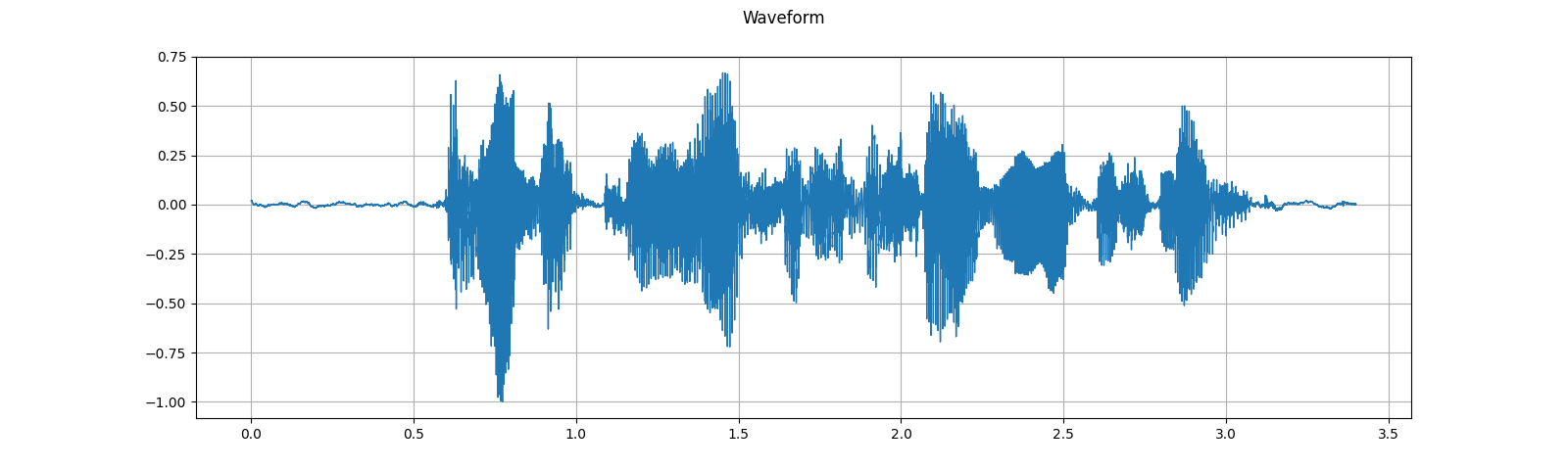
输出:

Sample Rate: 16000
Shape: (1, 54400)
Dtype: torch.float32
 - Max:      0.668
 - Min:     -1.000
 - Mean:     0.000
 - Std Dev:  0.122

tensor([[0.0183, 0.0180, 0.0180,  ..., 0.0018, 0.0019, 0.0032]])

<IPython.lib.display.Audio object>

从类文件对象加载

torchaudio 的 I/O 函数现在支持类文件对象。这使得可以从本地文件系统以外的位置获取音频数据并同时进行解码。以下示例说明了这一点。

# Load audio data as HTTP request
with requests.get(SAMPLE_WAV_SPEECH_URL, stream=True) as response:
  waveform, sample_rate = torchaudio.load(response.raw)
plot_specgram(waveform, sample_rate, title="HTTP datasource")

# Load audio from tar file
with tarfile.open(SAMPLE_TAR_PATH, mode='r') as tarfile_:
  fileobj = tarfile_.extractfile(SAMPLE_TAR_ITEM)
  waveform, sample_rate = torchaudio.load(fileobj)
plot_specgram(waveform, sample_rate, title="TAR file")

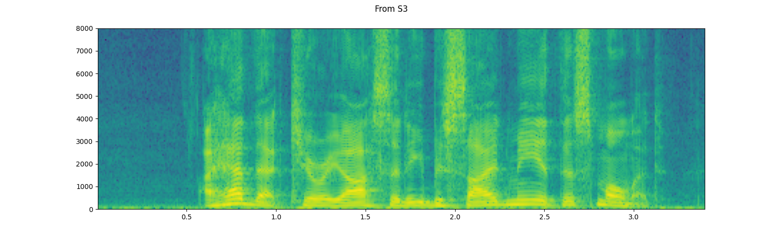
# Load audio from S3
client = boto3.client('s3', config=Config(signature_version=UNSIGNED))
response = client.get_object(Bucket=S3_BUCKET, Key=S3_KEY)
waveform, sample_rate = torchaudio.load(response['Body'])
plot_specgram(waveform, sample_rate, title="From S3")

• 
• 
• 

切片技巧

提供 num_frames 和 frame_offset 参数将在解码时切片生成的张量对象。

同样的结果可以通过常规的Tensor切片实现， （即waveform[:, frame_offset:frame_offset+num_frames]）然而， 提供num_frames和frame_offset参数更为高效。

这是因为该函数在完成解码请求的帧后将停止数据采集和解码。当音频数据通过网络传输时，这是有利的，因为一旦获取到必要数量的数据，数据传输就会停止。

以下示例说明了这一点；

# Illustration of two different decoding methods.
# The first one will fetch all the data and decode them, while
# the second one will stop fetching data once it completes decoding.
# The resulting waveforms are identical.

frame_offset, num_frames = 16000, 16000  # Fetch and decode the 1 - 2 seconds

print("Fetching all the data...")
with requests.get(SAMPLE_WAV_SPEECH_URL, stream=True) as response:
  waveform1, sample_rate1 = torchaudio.load(response.raw)
  waveform1 = waveform1[:, frame_offset:frame_offset+num_frames]
  print(f" - Fetched {response.raw.tell()} bytes")

print("Fetching until the requested frames are available...")
with requests.get(SAMPLE_WAV_SPEECH_URL, stream=True) as response:
  waveform2, sample_rate2 = torchaudio.load(
      response.raw, frame_offset=frame_offset, num_frames=num_frames)
  print(f" - Fetched {response.raw.tell()} bytes")

print("Checking the resulting waveform ... ", end="")
assert (waveform1 == waveform2).all()
print("matched!")

输出:

Fetching all the data...
 - Fetched 108844 bytes
Fetching until the requested frames are available...
 - Fetched 65580 bytes
Checking the resulting waveform ... matched!

将音频保存到文件

为了保存可以被常见应用程序解释的音频数据格式，你可以使用torchaudio.save。

此函数接受类似路径的对象和类似文件的对象。

当传递类似文件的对象时，您还需要提供format参数，以便函数知道应该使用哪种格式。在传递类似路径的对象时，函数将根据扩展名确定格式。如果您要保存到没有扩展名的文件，则需要提供format参数。

当保存为WAV格式时，float32张量的默认编码是32位浮点PCM。你可以提供encoding和bits_per_sample参数来改变这一点。例如，要以16位有符号整数PCM保存数据，你可以执行以下操作。

注意 以较低位深度的编码保存数据会减小生成的文件大小，但会损失精度。

waveform, sample_rate = get_sample()
print_stats(waveform, sample_rate=sample_rate)

# Save without any encoding option.
# The function will pick up the encoding which
# the provided data fit
path = "save_example_default.wav"
torchaudio.save(path, waveform, sample_rate)
inspect_file(path)

# Save as 16-bit signed integer Linear PCM
# The resulting file occupies half the storage but loses precision
path = "save_example_PCM_S16.wav"
torchaudio.save(
    path, waveform, sample_rate,
    encoding="PCM_S", bits_per_sample=16)
inspect_file(path)

输出:

Sample Rate: 44100
Shape: (1, 109368)
Dtype: torch.float32
 - Max:      0.508
 - Min:     -0.449
 - Mean:    -0.000
 - Std Dev:  0.122

tensor([[0.0027, 0.0063, 0.0092,  ..., 0.0032, 0.0047, 0.0052]])

----------
Source: save_example_default.wav
----------
 - File size: 437530 bytes
 - AudioMetaData(sample_rate=44100, num_frames=109368, num_channels=1, bits_per_sample=32, encoding=PCM_F)
----------
Source: save_example_PCM_S16.wav
----------
 - File size: 218780 bytes
 - AudioMetaData(sample_rate=44100, num_frames=109368, num_channels=1, bits_per_sample=16, encoding=PCM_S)

torchaudio.save 也可以处理其他格式。举几个例子；

waveform, sample_rate = get_sample(resample=8000)

formats = [
  "mp3",
  "flac",
  "vorbis",
  "sph",
  "amb",
  "amr-nb",
  "gsm",
]

for format in formats:
  path = f"save_example.{format}"
  torchaudio.save(path, waveform, sample_rate, format=format)
  inspect_file(path)

输出:

----------
Source: save_example.mp3
----------
 - File size: 2664 bytes
 - AudioMetaData(sample_rate=8000, num_frames=21312, num_channels=1, bits_per_sample=0, encoding=MP3)
----------
Source: save_example.flac
----------
 - File size: 47315 bytes
 - AudioMetaData(sample_rate=8000, num_frames=19840, num_channels=1, bits_per_sample=24, encoding=FLAC)
----------
Source: save_example.vorbis
----------
 - File size: 9967 bytes
 - AudioMetaData(sample_rate=8000, num_frames=19840, num_channels=1, bits_per_sample=0, encoding=VORBIS)
----------
Source: save_example.sph
----------
 - File size: 80384 bytes
 - AudioMetaData(sample_rate=8000, num_frames=19840, num_channels=1, bits_per_sample=32, encoding=PCM_S)
----------
Source: save_example.amb
----------
 - File size: 79418 bytes
 - AudioMetaData(sample_rate=8000, num_frames=19840, num_channels=1, bits_per_sample=32, encoding=PCM_F)
----------
Source: save_example.amr-nb
----------
 - File size: 1618 bytes
 - AudioMetaData(sample_rate=8000, num_frames=19840, num_channels=1, bits_per_sample=0, encoding=AMR_NB)
----------
Source: save_example.gsm
----------
 - File size: 4092 bytes
 - AudioMetaData(sample_rate=8000, num_frames=0, num_channels=1, bits_per_sample=0, encoding=GSM)

保存到类文件对象

与其他I/O函数类似，您可以将音频保存到类似文件的对象中。当保存到类似文件的对象时，format参数是必需的。

waveform, sample_rate = get_sample()

# Saving to Bytes buffer
buffer_ = io.BytesIO()
torchaudio.save(buffer_, waveform, sample_rate, format="wav")

buffer_.seek(0)
print(buffer_.read(16))

输出:

b'RIFF\x12\xad\x06\x00WAVEfmt '

重采样

要将音频波形从一个频率重新采样到另一个频率，你可以使用 transforms.Resample 或 functional.resample。 transforms.Resample 预先计算并缓存用于重新采样的内核，而 functional.resample 则是在运行时计算它，因此如果使用相同的参数重新采样多个波形， 使用 transforms.Resample 将会加速（参见基准测试部分）。

两种重采样方法都使用带限sinc插值来计算任意时间步长的信号值。实现涉及卷积，因此我们可以利用GPU/多线程来提高性能。当在多个子进程中使用重采样时，例如使用多个工作进程进行数据加载，您的应用程序可能会创建比系统能够有效处理的更多线程。在这种情况下，设置torch.set_num_threads(1)可能会有所帮助。

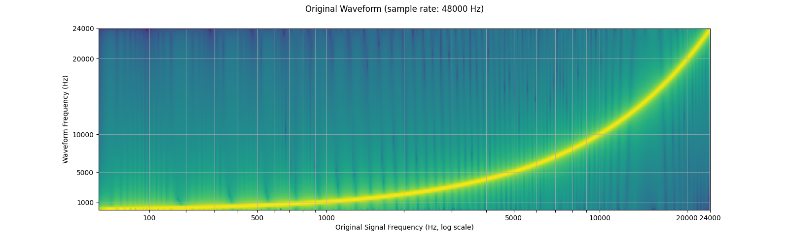
因为有限数量的样本只能代表有限数量的频率，重采样不会产生完美的结果，可以使用各种参数来控制其质量和计算速度。我们通过对数正弦扫频进行重采样来展示这些特性，这是一种频率随时间呈指数增长的正弦波。

下面的频谱图显示了信号的频率表示，其中x轴标签对应于原始波形的频率（以对数刻度表示），y轴对应于绘制波形的频率，颜色强度表示振幅。

sample_rate = 48000
resample_rate = 32000

waveform = get_sine_sweep(sample_rate)
plot_sweep(waveform, sample_rate, title="Original Waveform")
play_audio(waveform, sample_rate)

resampler = T.Resample(sample_rate, resample_rate, dtype=waveform.dtype)
resampled_waveform = resampler(waveform)
plot_sweep(resampled_waveform, resample_rate, title="Resampled Waveform")
play_audio(waveform, sample_rate)

• 
• 

输出:

<IPython.lib.display.Audio object>
<IPython.lib.display.Audio object>

使用参数控制重采样质量

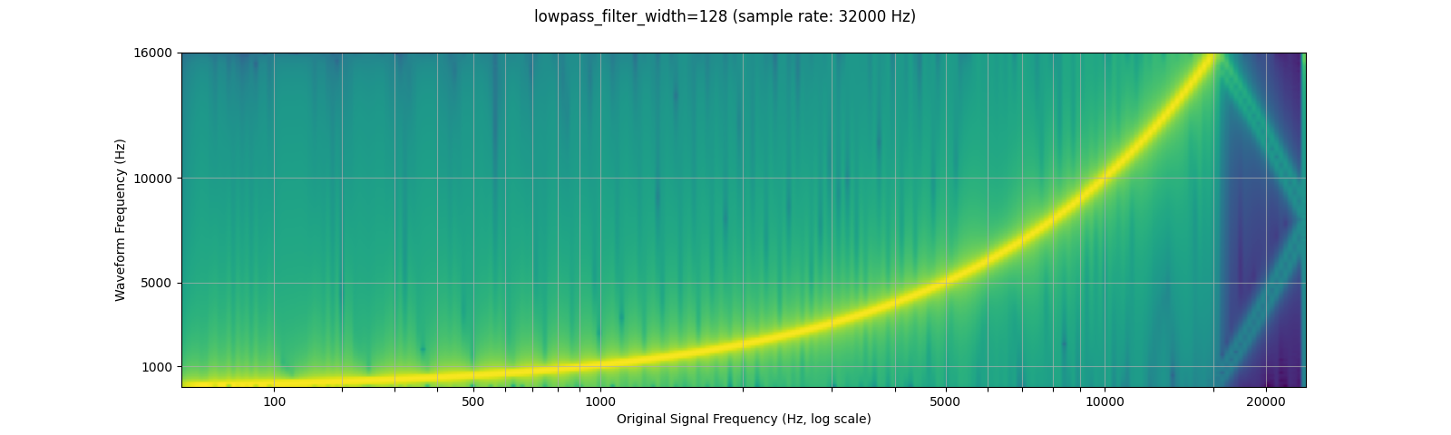
低通滤波器宽度

由于用于插值的滤波器无限延伸，lowpass_filter_width 参数用于控制用于窗口插值的滤波器的宽度。它也被称为零交叉数，因为插值在每个时间单位都通过零。使用较大的 lowpass_filter_width 可以提供更锐利、更精确的滤波器，但计算成本更高。

sample_rate = 48000
resample_rate = 32000

resampled_waveform = F.resample(waveform, sample_rate, resample_rate, lowpass_filter_width=6)
plot_sweep(resampled_waveform, resample_rate, title="lowpass_filter_width=6")

resampled_waveform = F.resample(waveform, sample_rate, resample_rate, lowpass_filter_width=128)
plot_sweep(resampled_waveform, resample_rate, title="lowpass_filter_width=128")

• 
• 

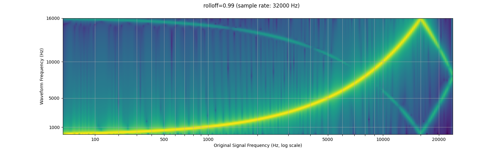
Rolloff

rolloff 参数表示为奈奎斯特频率的一部分，奈奎斯特频率是给定有限采样率可表示的最大频率。rolloff 决定了低通滤波器的截止频率，并控制混叠的程度，混叠发生在高于奈奎斯特的频率被映射到较低频率时。因此，较低的 rolloff 会减少混叠的量，但也会减少一些较高频率。

sample_rate = 48000
resample_rate = 32000

resampled_waveform = F.resample(waveform, sample_rate, resample_rate, rolloff=0.99)
plot_sweep(resampled_waveform, resample_rate, title="rolloff=0.99")

resampled_waveform = F.resample(waveform, sample_rate, resample_rate, rolloff=0.8)
plot_sweep(resampled_waveform, resample_rate, title="rolloff=0.8")

• 
• 

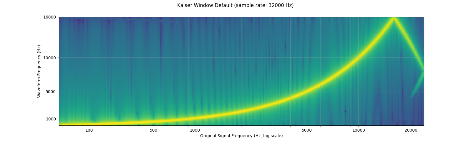
窗口函数

默认情况下，torchaudio的重采样使用汉恩窗口滤波器，这是一个加权余弦函数。它还支持凯撒窗口，这是一个接近最优的窗口函数，包含一个额外的beta参数，允许设计滤波器的平滑度和脉冲宽度。这可以通过resampling_method参数来控制。

sample_rate = 48000
resample_rate = 32000

resampled_waveform = F.resample(waveform, sample_rate, resample_rate, resampling_method="sinc_interpolation")
plot_sweep(resampled_waveform, resample_rate, title="Hann Window Default")

resampled_waveform = F.resample(waveform, sample_rate, resample_rate, resampling_method="kaiser_window")
plot_sweep(resampled_waveform, resample_rate, title="Kaiser Window Default")

• 
• 

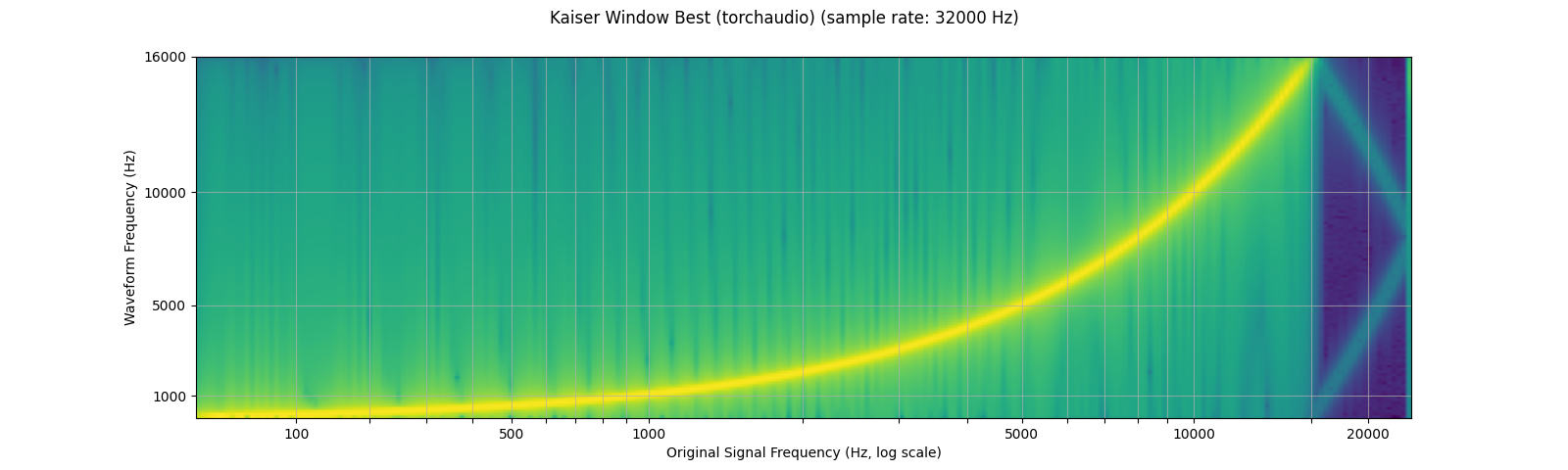
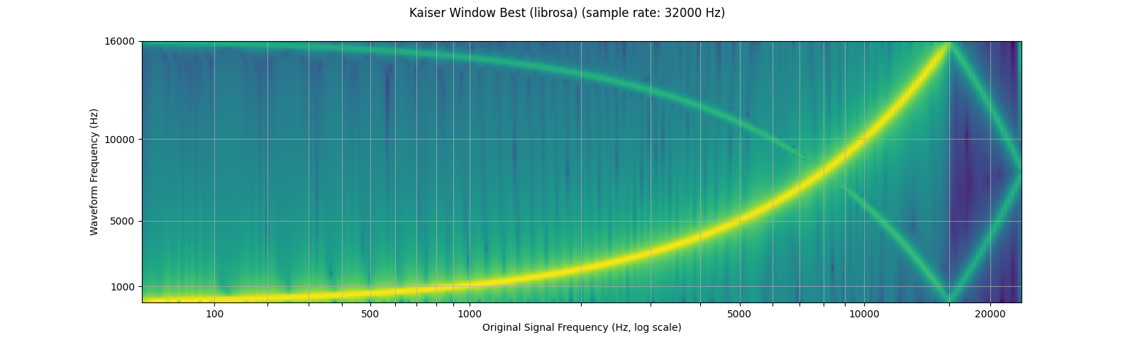
与librosa的比较

torchaudio的重采样函数可以用于产生类似于librosa（resampy）的kaiser窗口重采样的结果，但会有一些噪声。

sample_rate = 48000
resample_rate = 32000

### kaiser_best
resampled_waveform = F.resample(
    waveform,
    sample_rate,
    resample_rate,
    lowpass_filter_width=64,
    rolloff=0.9475937167399596,
    resampling_method="kaiser_window",
    beta=14.769656459379492
)
plot_sweep(resampled_waveform, resample_rate, title="Kaiser Window Best (torchaudio)")

librosa_resampled_waveform = torch.from_numpy(
    librosa.resample(waveform.squeeze().numpy(), sample_rate, resample_rate, res_type='kaiser_best')).unsqueeze(0)
plot_sweep(librosa_resampled_waveform, resample_rate, title="Kaiser Window Best (librosa)")

mse = torch.square(resampled_waveform - librosa_resampled_waveform).mean().item()
print("torchaudio and librosa kaiser best MSE:", mse)

### kaiser_fast
resampled_waveform = F.resample(
    waveform,
    sample_rate,
    resample_rate,
    lowpass_filter_width=16,
    rolloff=0.85,
    resampling_method="kaiser_window",
    beta=8.555504641634386
)
plot_specgram(resampled_waveform, resample_rate, title="Kaiser Window Fast (torchaudio)")

librosa_resampled_waveform = torch.from_numpy(
    librosa.resample(waveform.squeeze().numpy(), sample_rate, resample_rate, res_type='kaiser_fast')).unsqueeze(0)
plot_sweep(librosa_resampled_waveform, resample_rate, title="Kaiser Window Fast (librosa)")

mse = torch.square(resampled_waveform - librosa_resampled_waveform).mean().item()
print("torchaudio and librosa kaiser fast MSE:", mse)

• 
• 
• 
• 

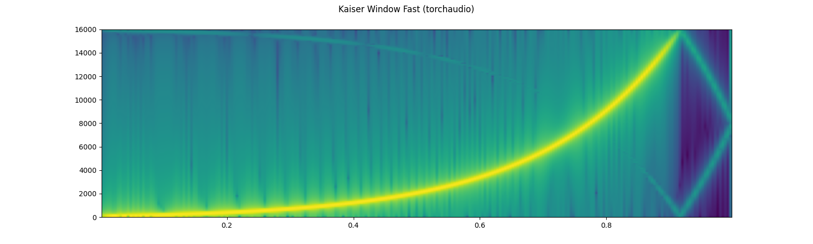
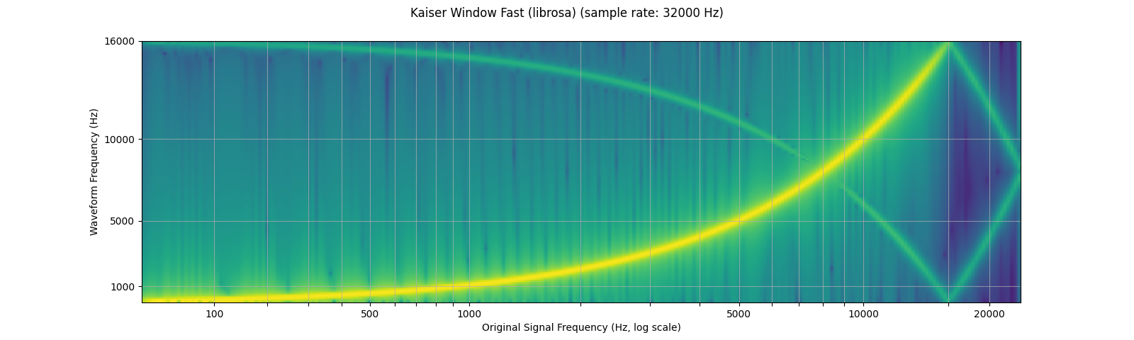
输出:

torchaudio and librosa kaiser best MSE: 2.080690115365992e-06
torchaudio and librosa kaiser fast MSE: 2.5200744248601027e-05

性能基准测试

以下是两种采样率之间下采样和上采样波形的基准测试。我们展示了lowpass_filter_wdith、窗口类型和采样率可能对性能的影响。此外，我们还提供了与librosa的kaiser_best和kaiser_fast在torchaudio中使用相应参数的比较。

详细说明结果：

• a larger lowpass_filter_width results in a larger resampling kernel, and therefore increases computation time for both the kernel computation and convolution
• using kaiser_window results in longer computation times than the default sinc_interpolation because it is more complex to compute the intermediate window values - a large GCD between the sample and resample rate will result in a simplification that allows for a smaller kernel and faster kernel computation.

configs = {
    "downsample (48 -> 44.1 kHz)": [48000, 44100],
    "downsample (16 -> 8 kHz)": [16000, 8000],
    "upsample (44.1 -> 48 kHz)": [44100, 48000],
    "upsample (8 -> 16 kHz)": [8000, 16000],
}

for label in configs:
  times, rows = [], []
  sample_rate = configs[label][0]
  resample_rate = configs[label][1]
  waveform = get_sine_sweep(sample_rate)

  # sinc 64 zero-crossings
  f_time = benchmark_resample("functional", waveform, sample_rate, resample_rate, lowpass_filter_width=64)
  t_time = benchmark_resample("transforms", waveform, sample_rate, resample_rate, lowpass_filter_width=64)
  times.append([None, 1000 * f_time, 1000 * t_time])
  rows.append(f"sinc (width 64)")

  # sinc 6 zero-crossings
  f_time = benchmark_resample("functional", waveform, sample_rate, resample_rate, lowpass_filter_width=16)
  t_time = benchmark_resample("transforms", waveform, sample_rate, resample_rate, lowpass_filter_width=16)
  times.append([None, 1000 * f_time, 1000 * t_time])
  rows.append(f"sinc (width 16)")

  # kaiser best
  lib_time = benchmark_resample("librosa", waveform, sample_rate, resample_rate, librosa_type="kaiser_best")
  f_time = benchmark_resample(
      "functional",
      waveform,
      sample_rate,
      resample_rate,
      lowpass_filter_width=64,
      rolloff=0.9475937167399596,
      resampling_method="kaiser_window",
      beta=14.769656459379492)
  t_time = benchmark_resample(
      "transforms",
      waveform,
      sample_rate,
      resample_rate,
      lowpass_filter_width=64,
      rolloff=0.9475937167399596,
      resampling_method="kaiser_window",
      beta=14.769656459379492)
  times.append([1000 * lib_time, 1000 * f_time, 1000 * t_time])
  rows.append(f"kaiser_best")

  # kaiser fast
  lib_time = benchmark_resample("librosa", waveform, sample_rate, resample_rate, librosa_type="kaiser_fast")
  f_time = benchmark_resample(
      "functional",
      waveform,
      sample_rate,
      resample_rate,
      lowpass_filter_width=16,
      rolloff=0.85,
      resampling_method="kaiser_window",
      beta=8.555504641634386)
  t_time = benchmark_resample(
      "transforms",
      waveform,
      sample_rate,
      resample_rate,
      lowpass_filter_width=16,
      rolloff=0.85,
      resampling_method="kaiser_window",
      beta=8.555504641634386)
  times.append([1000 * lib_time, 1000 * f_time, 1000 * t_time])
  rows.append(f"kaiser_fast")

  df = pd.DataFrame(times,
                    columns=["librosa", "functional", "transforms"],
                    index=rows)
  df.columns = pd.MultiIndex.from_product([[f"{label} time (ms)"],df.columns])
  display(df.round(2))

输出:

downsample (48 -> 44.1 kHz) time (ms)
                                              librosa functional transforms
sinc (width 64)                                   NaN      18.17       0.42
sinc (width 16)                                   NaN      16.67       0.37
kaiser_best                                     58.26      25.67       0.42
kaiser_fast                                      9.66      23.96       0.38
                downsample (16 -> 8 kHz) time (ms)
                                           librosa functional transforms
sinc (width 64)                                NaN       1.71       0.56
sinc (width 16)                                NaN       0.46       0.28
kaiser_best                                  20.48       0.94       0.52
kaiser_fast                                   4.26       0.56       0.28
                upsample (44.1 -> 48 kHz) time (ms)
                                            librosa functional transforms
sinc (width 64)                                 NaN      19.58       0.45
sinc (width 16)                                 NaN      18.19       0.42
kaiser_best                                   61.97      27.90       0.46
kaiser_fast                                    9.71      25.77       0.42
                upsample (8 -> 16 kHz) time (ms)
                                         librosa functional transforms
sinc (width 64)                              NaN       0.79       0.39
sinc (width 16)                              NaN       0.57       0.25
kaiser_best                                20.75       0.88       0.41
kaiser_fast                                 4.24       0.70       0.27

数据增强

torchaudio 提供了多种增强音频数据的方法。

应用效果和过滤

torchaudio.sox_effects 模块提供了直接在张量对象和文件对象音频源上应用类似 sox 命令的过滤器的方法。

为此有两个函数；

• torchaudio.sox_effects.apply_effects_tensor for applying effects on Tensor
• torchaudio.sox_effects.apply_effects_file for applying effects on other audio source

两个函数都以List[List[str]]的形式生效。这主要对应于sox命令的工作方式，但需要注意的是，sox命令会自动添加一些效果，而torchaudio的实现则不会这样做。

有关可用效果的列表，请参阅sox文档。

提示 如果您需要动态加载并重新采样音频数据， 那么可以使用 torchaudio.sox_effects.apply_effects_file 并配合 "rate" 效果。

注意 apply_effects_file 接受类似文件的对象或路径对象。类似于 torchaudio.load，当无法从文件扩展名或头部检测到音频格式时，您可以提供 format 参数来指定音频源的格式。

注意 这个过程是不可微分的。

# Load the data
waveform1, sample_rate1 = get_sample(resample=16000)

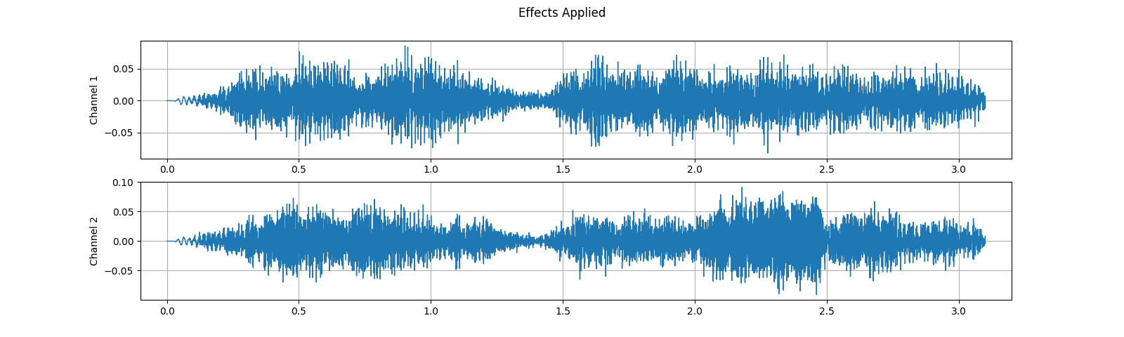
# Define effects
effects = [
  ["lowpass", "-1", "300"], # apply single-pole lowpass filter
  ["speed", "0.8"],  # reduce the speed
                     # This only changes sample rate, so it is necessary to
                     # add `rate` effect with original sample rate after this.
  ["rate", f"{sample_rate1}"],
  ["reverb", "-w"],  # Reverbration gives some dramatic feeling
]

# Apply effects
waveform2, sample_rate2 = torchaudio.sox_effects.apply_effects_tensor(
    waveform1, sample_rate1, effects)

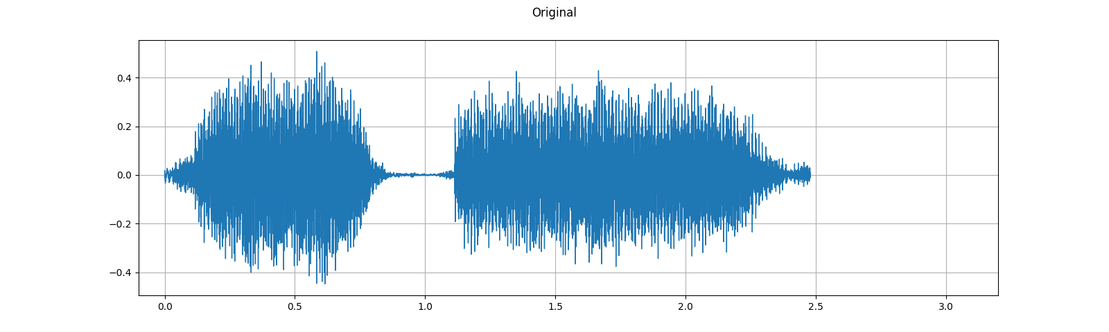
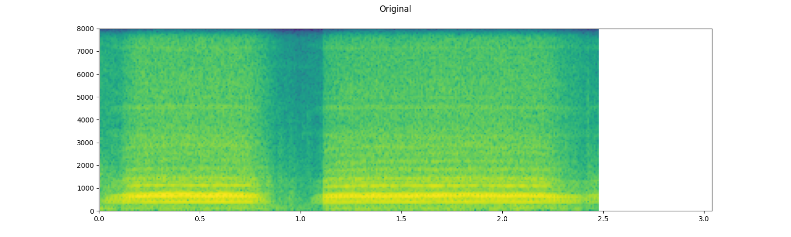
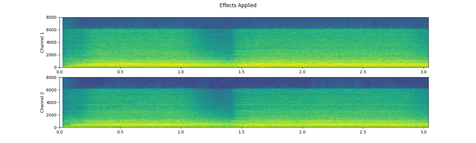
plot_waveform(waveform1, sample_rate1, title="Original", xlim=(-.1, 3.2))
plot_waveform(waveform2, sample_rate2, title="Effects Applied", xlim=(-.1, 3.2))
print_stats(waveform1, sample_rate=sample_rate1, src="Original")
print_stats(waveform2, sample_rate=sample_rate2, src="Effects Applied")

• 
• 

输出:

----------
Source: Original
----------
Sample Rate: 16000
Shape: (1, 39680)
Dtype: torch.float32
 - Max:      0.507
 - Min:     -0.448
 - Mean:    -0.000
 - Std Dev:  0.122

tensor([[ 0.0007,  0.0076,  0.0122,  ..., -0.0049, -0.0025,  0.0020]])

----------
Source: Effects Applied
----------
Sample Rate: 16000
Shape: (2, 49600)
Dtype: torch.float32
 - Max:      0.091
 - Min:     -0.091
 - Mean:    -0.000
 - Std Dev:  0.021

tensor([[0.0000, 0.0000, 0.0000,  ..., 0.0069, 0.0058, 0.0045],
        [0.0000, 0.0000, 0.0000,  ..., 0.0085, 0.0085, 0.0085]])

请注意，经过效果处理后，帧数和通道数与原始音频不同。让我们来听一下音频。听起来是不是更加戏剧化了？

plot_specgram(waveform1, sample_rate1, title="Original", xlim=(0, 3.04))
play_audio(waveform1, sample_rate1)
plot_specgram(waveform2, sample_rate2, title="Effects Applied", xlim=(0, 3.04))
play_audio(waveform2, sample_rate2)

• 
• 

输出:

<IPython.lib.display.Audio object>
<IPython.lib.display.Audio object>

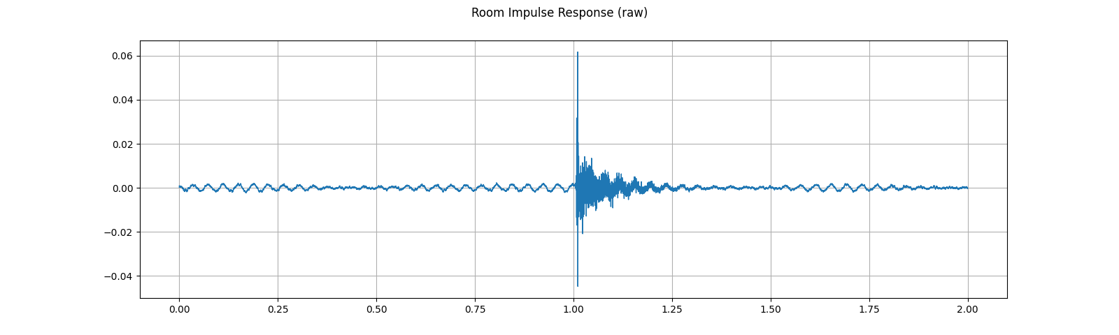
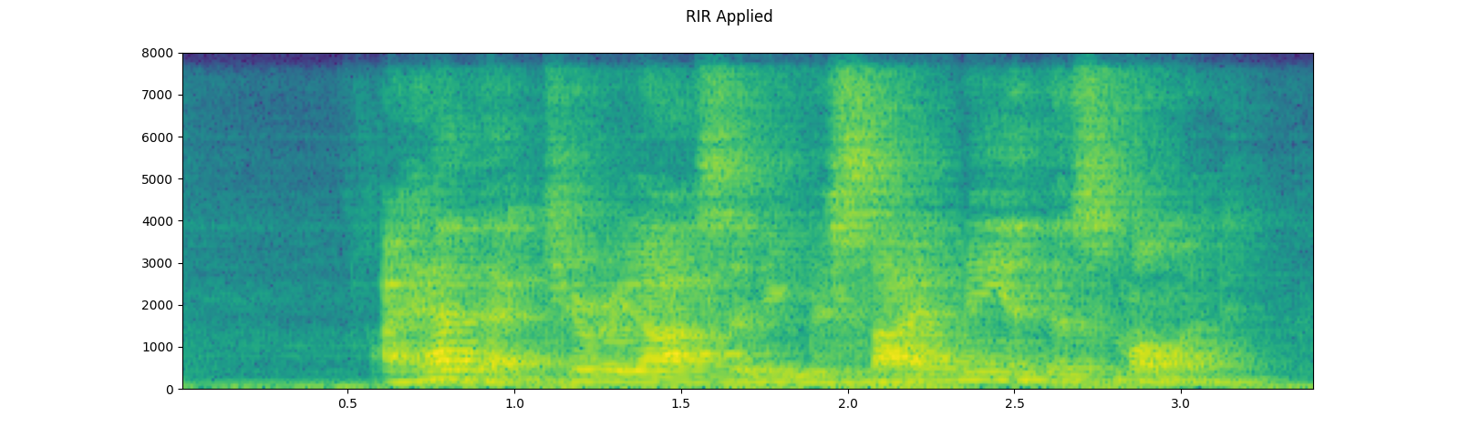
模拟房间混响

Convolution reverb 是一种技术，用于使干净的音频数据听起来像是在不同的环境中。

使用房间脉冲响应（RIR），我们可以使清晰的语音听起来像是在会议室中发出的。

对于这个过程，我们需要RIR数据。以下数据来自VOiCES数据集，但你可以自己录制一个。只需打开麦克风并拍手。

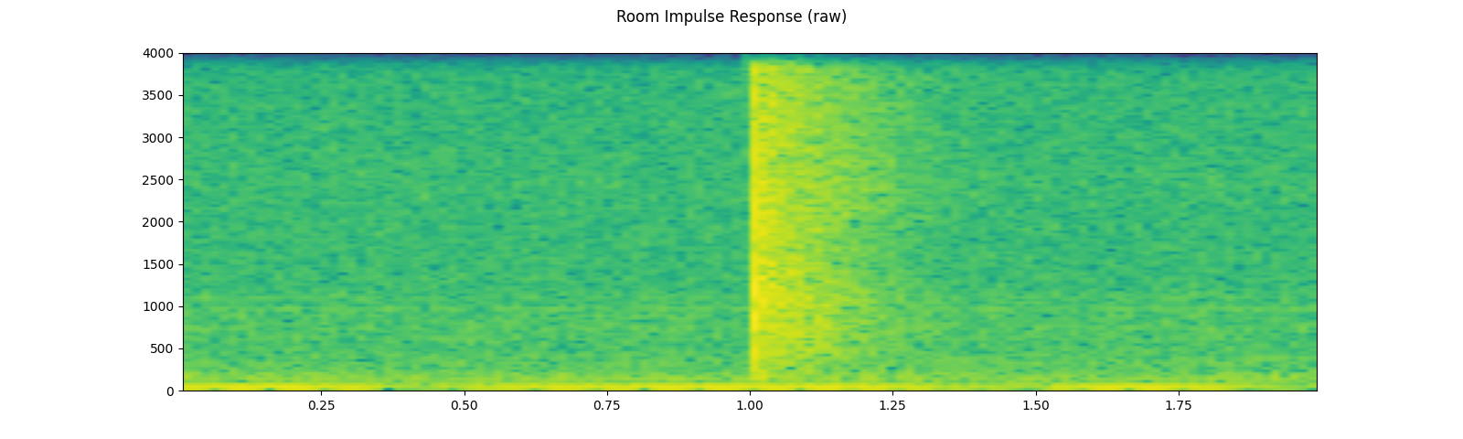
sample_rate = 8000

rir_raw, _ = get_rir_sample(resample=sample_rate)

plot_waveform(rir_raw, sample_rate, title="Room Impulse Response (raw)", ylim=None)
plot_specgram(rir_raw, sample_rate, title="Room Impulse Response (raw)")
play_audio(rir_raw, sample_rate)

• 
• 

输出:

<IPython.lib.display.Audio object>

首先，我们需要清理RIR。我们提取主要脉冲，归一化信号功率，然后翻转时间轴。

rir = rir_raw[:, int(sample_rate*1.01):int(sample_rate*1.3)]
rir = rir / torch.norm(rir, p=2)
rir = torch.flip(rir, [1])

print_stats(rir)
plot_waveform(rir, sample_rate, title="Room Impulse Response", ylim=None)

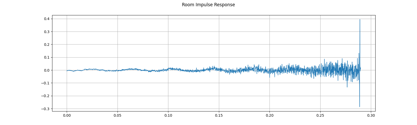
输出:

Shape: (1, 2320)
Dtype: torch.float32
 - Max:      0.395
 - Min:     -0.286
 - Mean:    -0.000
 - Std Dev:  0.021

tensor([[-0.0052, -0.0076, -0.0071,  ...,  0.0184,  0.0173,  0.0070]])

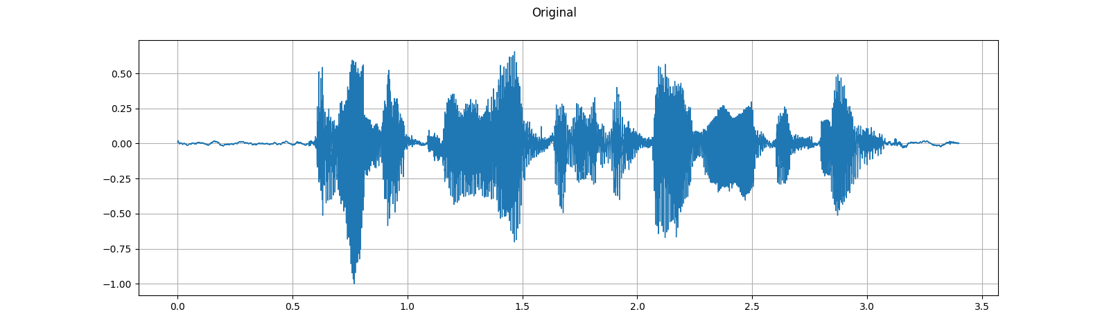
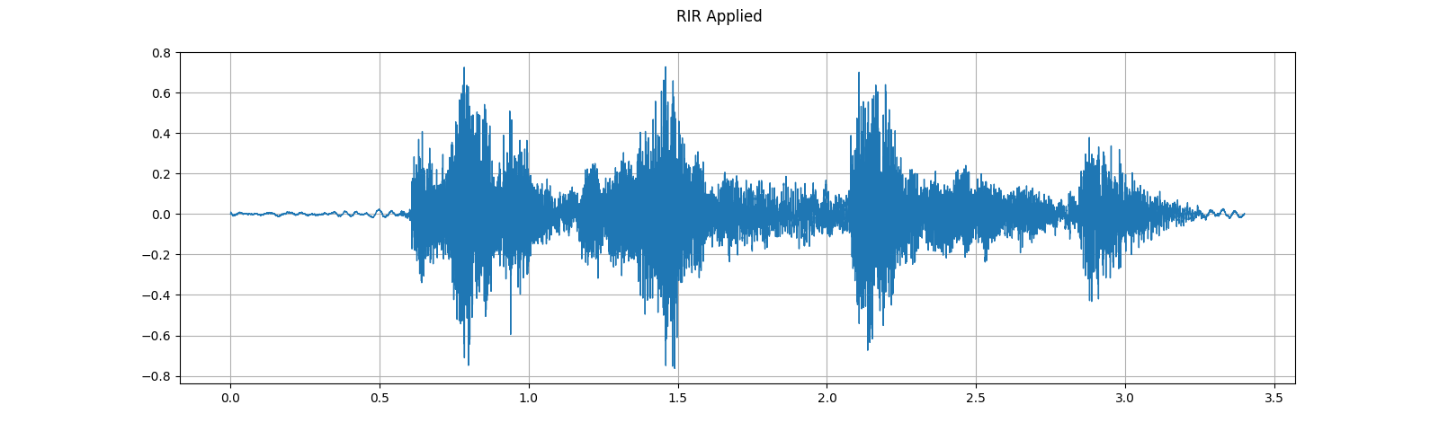
然后我们将语音信号与RIR滤波器进行卷积。

speech, _ = get_speech_sample(resample=sample_rate)

speech_ = torch.nn.functional.pad(speech, (rir.shape[1]-1, 0))
augmented = torch.nn.functional.conv1d(speech_[None, ...], rir[None, ...])[0]

plot_waveform(speech, sample_rate, title="Original", ylim=None)
plot_waveform(augmented, sample_rate, title="RIR Applied", ylim=None)

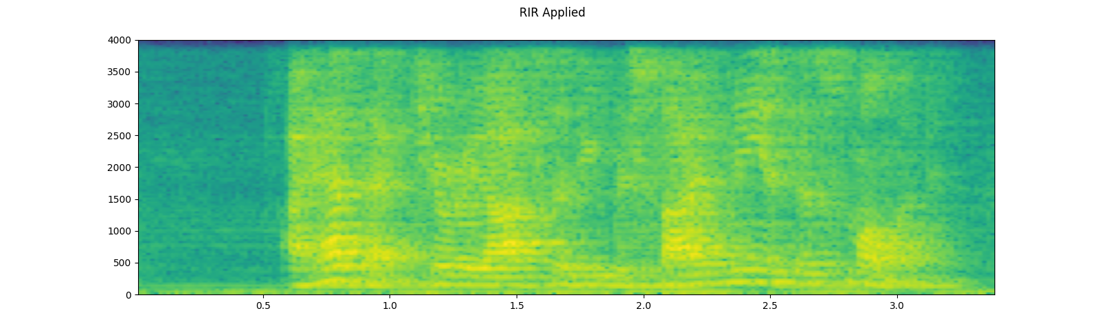
plot_specgram(speech, sample_rate, title="Original")
play_audio(speech, sample_rate)

plot_specgram(augmented, sample_rate, title="RIR Applied")
play_audio(augmented, sample_rate)

• 
• 
• 
• 

输出:

<IPython.lib.display.Audio object>
<IPython.lib.display.Audio object>

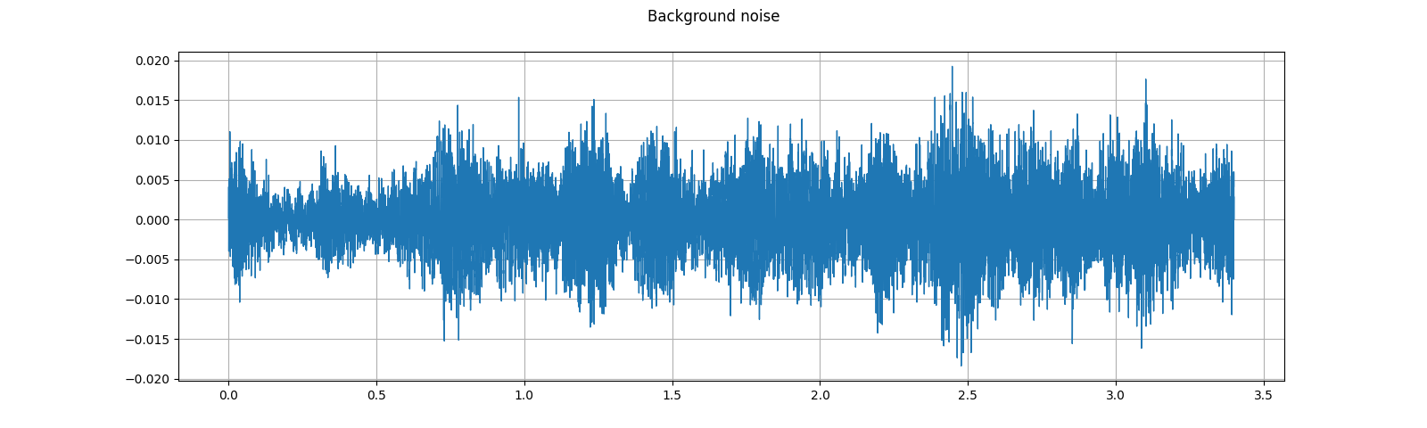
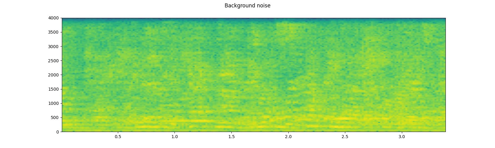
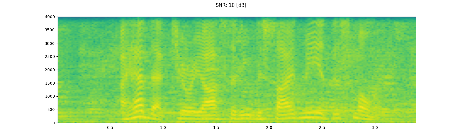
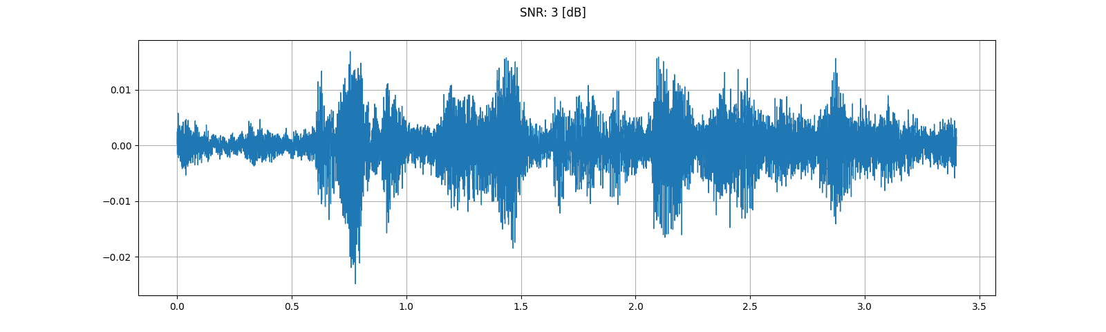
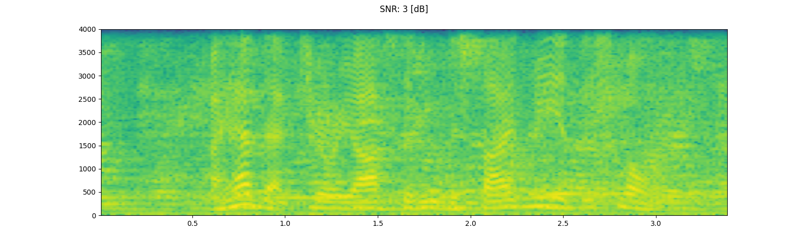
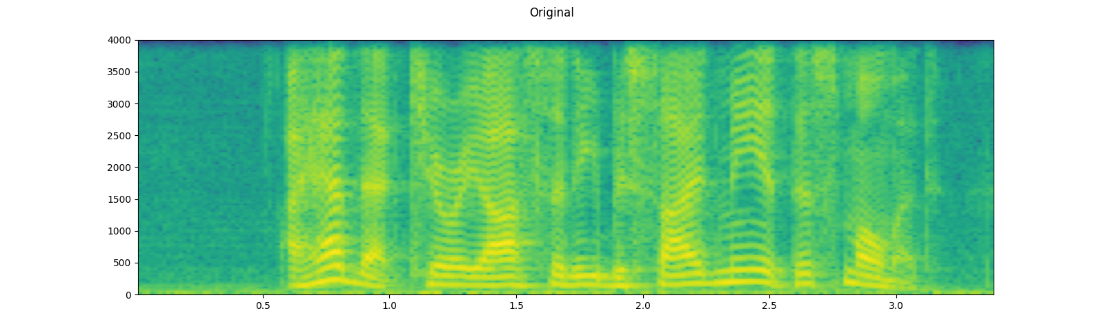
添加背景噪声

为了向音频数据添加背景噪声，您可以简单地将音频张量和噪声张量相加。调整噪声强度的常用方法是改变信噪比（SNR）。 [wikipedia]

\[\mathrm{SNR} = \frac{P_\mathrm{signal}}{P_\mathrm{noise}}\]

\[{\mathrm {SNR_{{dB}}}}=10\log _{{10}}\left({\mathrm {SNR}}\right)\]

sample_rate = 8000
speech, _ = get_speech_sample(resample=sample_rate)
noise, _ = get_noise_sample(resample=sample_rate)
noise = noise[:, :speech.shape[1]]

plot_waveform(noise, sample_rate, title="Background noise")
plot_specgram(noise, sample_rate, title="Background noise")
play_audio(noise, sample_rate)

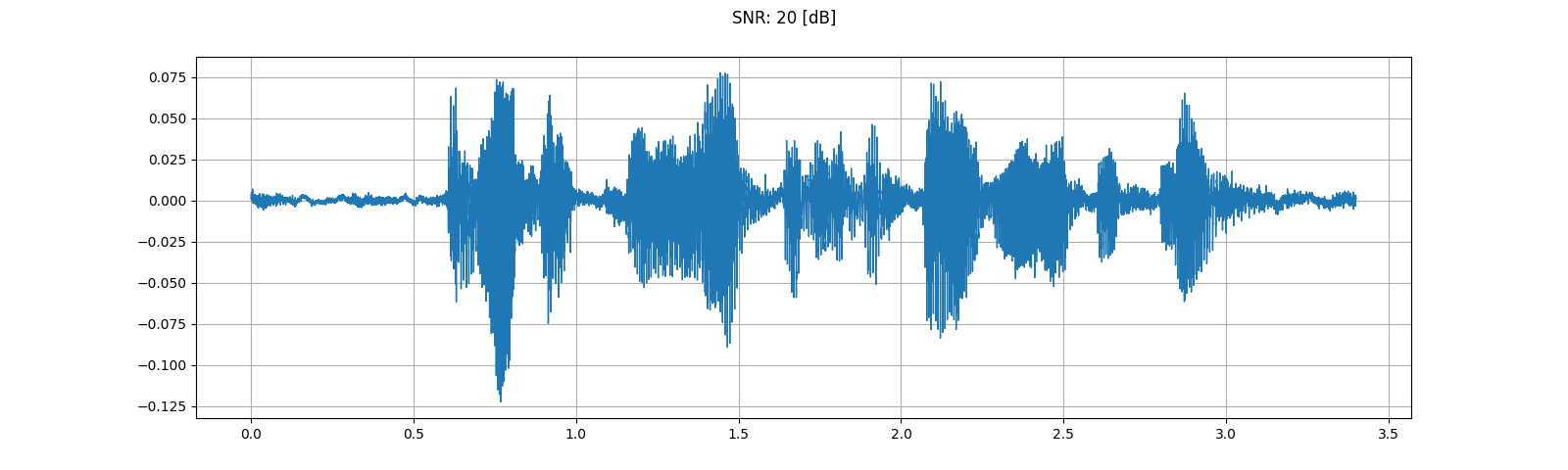
speech_power = speech.norm(p=2)
noise_power = noise.norm(p=2)

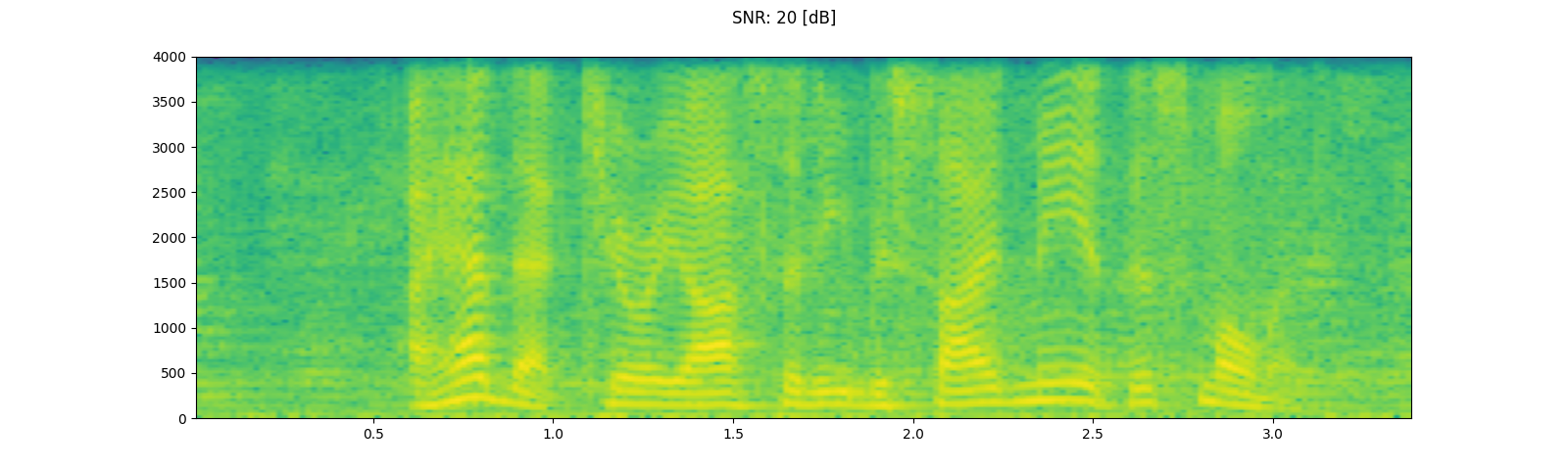
for snr_db in [20, 10, 3]:
  snr = math.exp(snr_db / 10)
  scale = snr * noise_power / speech_power
  noisy_speech = (scale * speech + noise) / 2

  plot_waveform(noisy_speech, sample_rate, title=f"SNR: {snr_db} [dB]")
  plot_specgram(noisy_speech, sample_rate, title=f"SNR: {snr_db} [dB]")
  play_audio(noisy_speech, sample_rate)

• 
• 
• 
• 
• 
• 
• 
• 

输出:

<IPython.lib.display.Audio object>
<IPython.lib.display.Audio object>
<IPython.lib.display.Audio object>
<IPython.lib.display.Audio object>

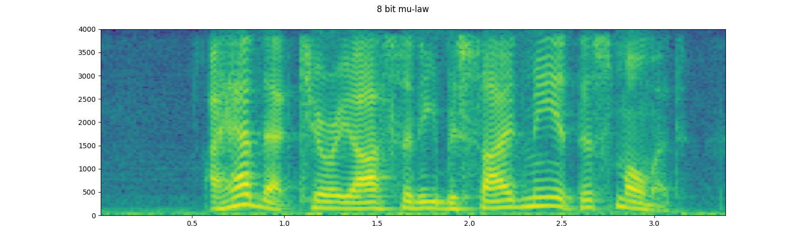
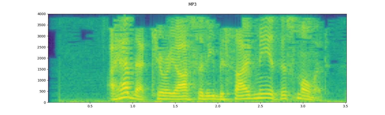
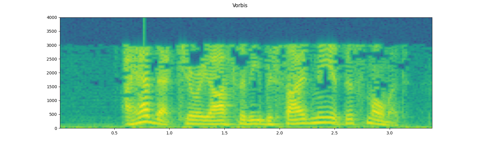
将编解码器应用于Tensor对象

torchaudio.functional.apply_codec 可以对 Tensor 对象应用编解码器。

注意 这个过程是不可微分的。

waveform, sample_rate = get_speech_sample(resample=8000)

plot_specgram(waveform, sample_rate, title="Original")
play_audio(waveform, sample_rate)

configs = [
    ({"format": "wav", "encoding": 'ULAW', "bits_per_sample": 8}, "8 bit mu-law"),
    ({"format": "gsm"}, "GSM-FR"),
    ({"format": "mp3", "compression": -9}, "MP3"),
    ({"format": "vorbis", "compression": -1}, "Vorbis"),
]
for param, title in configs:
  augmented = F.apply_codec(waveform, sample_rate, **param)
  plot_specgram(augmented, sample_rate, title=title)
  play_audio(augmented, sample_rate)

• 
• 
• 
• 
• 

输出:

<IPython.lib.display.Audio object>
<IPython.lib.display.Audio object>
<IPython.lib.display.Audio object>
<IPython.lib.display.Audio object>
<IPython.lib.display.Audio object>

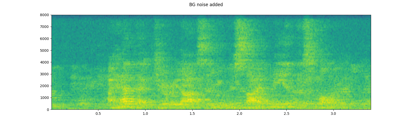
模拟电话录音

结合之前的技术，我们可以模拟出听起来像一个人在回声很大的房间里通过电话交谈，同时背景中有人说话的音频。

sample_rate = 16000
speech, _ = get_speech_sample(resample=sample_rate)

plot_specgram(speech, sample_rate, title="Original")
play_audio(speech, sample_rate)

# Apply RIR
rir, _ = get_rir_sample(resample=sample_rate, processed=True)
speech_ = torch.nn.functional.pad(speech, (rir.shape[1]-1, 0))
speech = torch.nn.functional.conv1d(speech_[None, ...], rir[None, ...])[0]

plot_specgram(speech, sample_rate, title="RIR Applied")
play_audio(speech, sample_rate)

# Add background noise
# Because the noise is recorded in the actual environment, we consider that
# the noise contains the acoustic feature of the environment. Therefore, we add
# the noise after RIR application.
noise, _ = get_noise_sample(resample=sample_rate)
noise = noise[:, :speech.shape[1]]

snr_db = 8
scale = math.exp(snr_db / 10) * noise.norm(p=2) / speech.norm(p=2)
speech = (scale * speech + noise) / 2

plot_specgram(speech, sample_rate, title="BG noise added")
play_audio(speech, sample_rate)

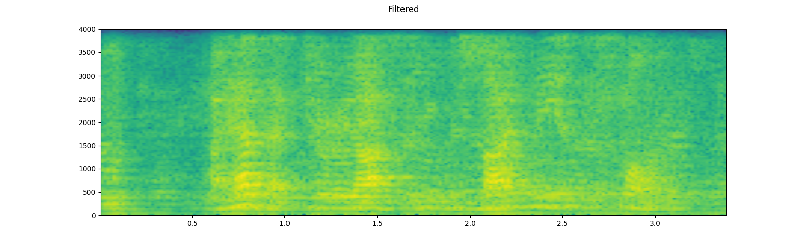
# Apply filtering and change sample rate
speech, sample_rate = torchaudio.sox_effects.apply_effects_tensor(
  speech,
  sample_rate,
  effects=[
      ["lowpass", "4000"],
      ["compand", "0.02,0.05", "-60,-60,-30,-10,-20,-8,-5,-8,-2,-8", "-8", "-7", "0.05"],
      ["rate", "8000"],
  ],
)

plot_specgram(speech, sample_rate, title="Filtered")
play_audio(speech, sample_rate)

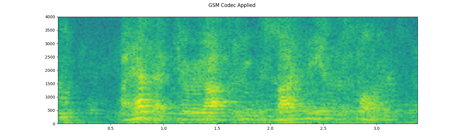
# Apply telephony codec
speech = F.apply_codec(speech, sample_rate, format="gsm")

plot_specgram(speech, sample_rate, title="GSM Codec Applied")
play_audio(speech, sample_rate)

• 
• 
• 
• 
• 

输出:

<IPython.lib.display.Audio object>
<IPython.lib.display.Audio object>
<IPython.lib.display.Audio object>
<IPython.lib.display.Audio object>
<IPython.lib.display.Audio object>

特征提取

torchaudio 实现了音频领域中常用的特征提取功能。它们可以在 torchaudio.functional 和 torchaudio.transforms 中找到。

functional 模块实现了作为独立函数的功能。它们是无状态的。

transforms 模块以面向对象的方式实现功能， 使用来自 functional 和 torch.nn.Module 的实现。

因为所有的转换都是torch.nn.Module的子类，它们可以使用TorchScript进行序列化。

有关可用功能的完整列表，请参阅文档。在本教程中，我们将探讨时域和频域之间的转换（Spectrogram，GriffinLim，MelSpectrogram）以及称为SpecAugment的增强技术。

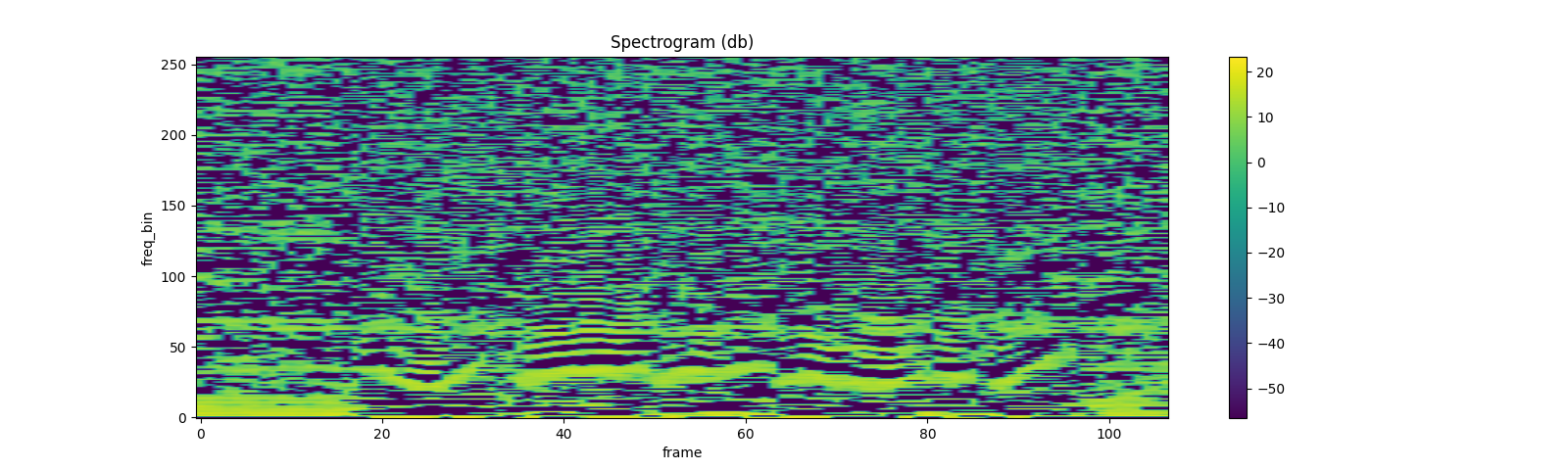
频谱图

要获取音频信号的频率表示，你可以使用 Spectrogram 变换。

waveform, sample_rate = get_speech_sample()

n_fft = 1024
win_length = None
hop_length = 512

# define transformation
spectrogram = T.Spectrogram(
    n_fft=n_fft,
    win_length=win_length,
    hop_length=hop_length,
    center=True,
    pad_mode="reflect",
    power=2.0,
)
# Perform transformation
spec = spectrogram(waveform)

print_stats(spec)
plot_spectrogram(spec[0], title='torchaudio')

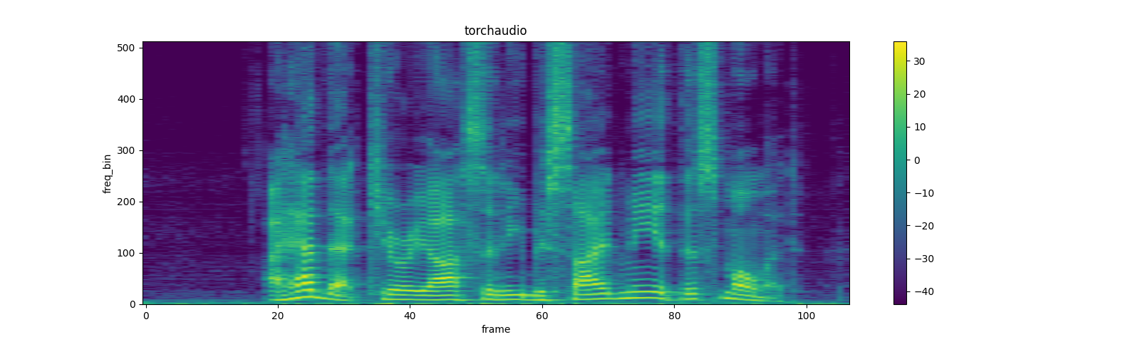
输出:

Shape: (1, 513, 107)
Dtype: torch.float32
 - Max:     4000.533
 - Min:      0.000
 - Mean:     5.726
 - Std Dev: 70.301

tensor([[[7.8743e+00, 4.4462e+00, 5.6781e-01,  ..., 2.7694e+01,
          8.9546e+00, 4.1289e+00],
         [7.1094e+00, 3.2595e+00, 7.3520e-01,  ..., 1.7141e+01,
          4.4812e+00, 8.0840e-01],
         [3.8374e+00, 8.2490e-01, 3.0779e-01,  ..., 1.8502e+00,
          1.1777e-01, 1.2369e-01],
         ...,
         [3.4708e-07, 1.0604e-05, 1.2395e-05,  ..., 7.4090e-06,
          8.2063e-07, 1.0176e-05],
         [4.7173e-05, 4.4329e-07, 3.9444e-05,  ..., 3.0622e-05,
          3.9735e-07, 8.1572e-06],
         [1.3221e-04, 1.6440e-05, 7.2536e-05,  ..., 5.4662e-05,
          1.1663e-05, 2.5758e-06]]])

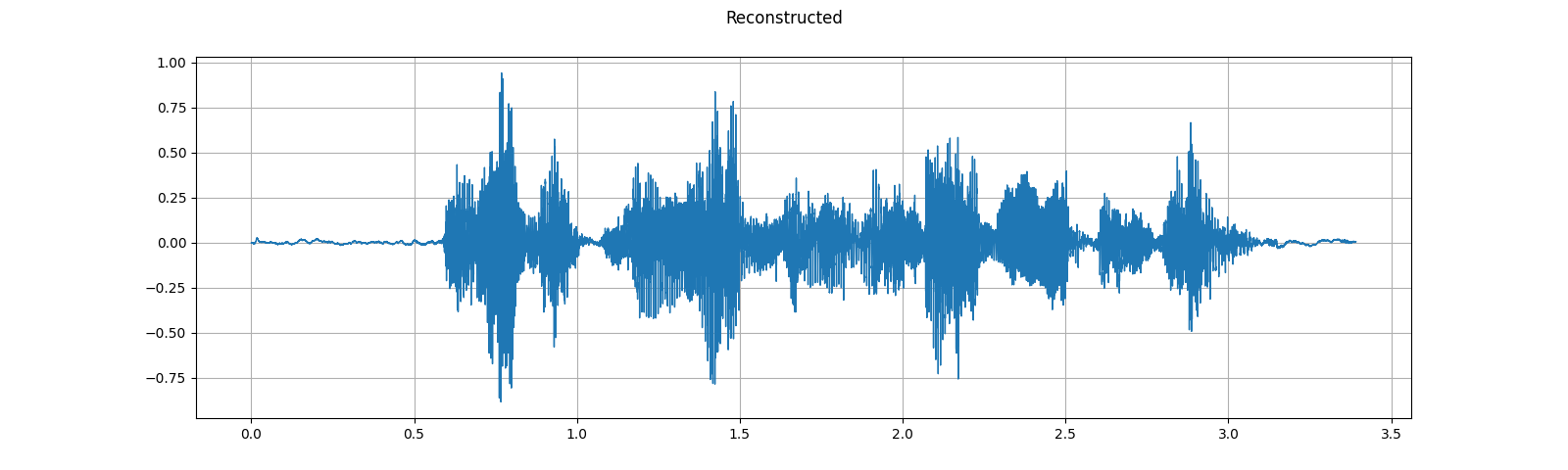
GriffinLim

要从频谱图中恢复波形，你可以使用 GriffinLim。

torch.random.manual_seed(0)
waveform, sample_rate = get_speech_sample()
plot_waveform(waveform, sample_rate, title="Original")
play_audio(waveform, sample_rate)

n_fft = 1024
win_length = None
hop_length = 512

spec = T.Spectrogram(
    n_fft=n_fft,
    win_length=win_length,
    hop_length=hop_length,
)(waveform)

griffin_lim = T.GriffinLim(
    n_fft=n_fft,
    win_length=win_length,
    hop_length=hop_length,
)
waveform = griffin_lim(spec)

plot_waveform(waveform, sample_rate, title="Reconstructed")
play_audio(waveform, sample_rate)

• 
• 

输出:

<IPython.lib.display.Audio object>
<IPython.lib.display.Audio object>

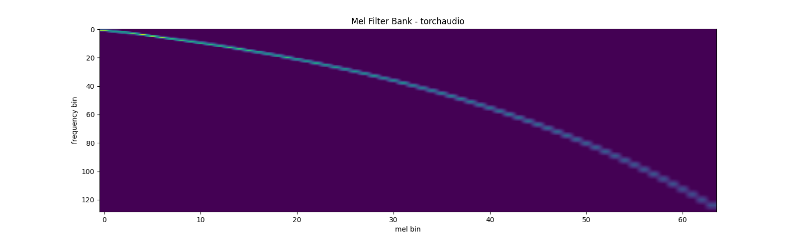
梅尔滤波器组

torchaudio.functional.create_fb_matrix 可以生成滤波器组 将频率仓转换为梅尔尺度仓。

由于此函数不需要输入音频/特征，因此在torchaudio.transforms中没有等效的转换。

n_fft = 256
n_mels = 64
sample_rate = 6000

mel_filters = F.create_fb_matrix(
    int(n_fft // 2 + 1),
    n_mels=n_mels,
    f_min=0.,
    f_max=sample_rate/2.,
    sample_rate=sample_rate,
    norm='slaney'
)
plot_mel_fbank(mel_filters, "Mel Filter Bank - torchaudio")

与librosa的比较

作为比较，这里是使用librosa获取梅尔滤波器组的等效方法。

mel_filters_librosa = librosa.filters.mel(
    sample_rate,
    n_fft,
    n_mels=n_mels,
    fmin=0.,
    fmax=sample_rate/2.,
    norm='slaney',
    htk=True,
).T

plot_mel_fbank(mel_filters_librosa, "Mel Filter Bank - librosa")

mse = torch.square(mel_filters - mel_filters_librosa).mean().item()
print('Mean Square Difference: ', mse)

输出:

Mean Square Difference:  3.795462323290159e-17

梅尔频谱图

梅尔尺度频谱图是频谱图和梅尔尺度转换的结合。在torchaudio中，有一个转换MelSpectrogram，它由Spectrogram和MelScale组成。

waveform, sample_rate = get_speech_sample()

n_fft = 1024
win_length = None
hop_length = 512
n_mels = 128

mel_spectrogram = T.MelSpectrogram(
    sample_rate=sample_rate,
    n_fft=n_fft,
    win_length=win_length,
    hop_length=hop_length,
    center=True,
    pad_mode="reflect",
    power=2.0,
    norm='slaney',
    onesided=True,
    n_mels=n_mels,
    mel_scale="htk",
)

melspec = mel_spectrogram(waveform)
plot_spectrogram(
    melspec[0], title="MelSpectrogram - torchaudio", ylabel='mel freq')

与librosa的比较

作为比较，这里是使用librosa获取梅尔频谱图的等效方法。

melspec_librosa = librosa.feature.melspectrogram(
    waveform.numpy()[0],
    sr=sample_rate,
    n_fft=n_fft,
    hop_length=hop_length,
    win_length=win_length,
    center=True,
    pad_mode="reflect",
    power=2.0,
    n_mels=n_mels,
    norm='slaney',
    htk=True,
)
plot_spectrogram(
    melspec_librosa, title="MelSpectrogram - librosa", ylabel='mel freq')

mse = torch.square(melspec - melspec_librosa).mean().item()
print('Mean Square Difference: ', mse)

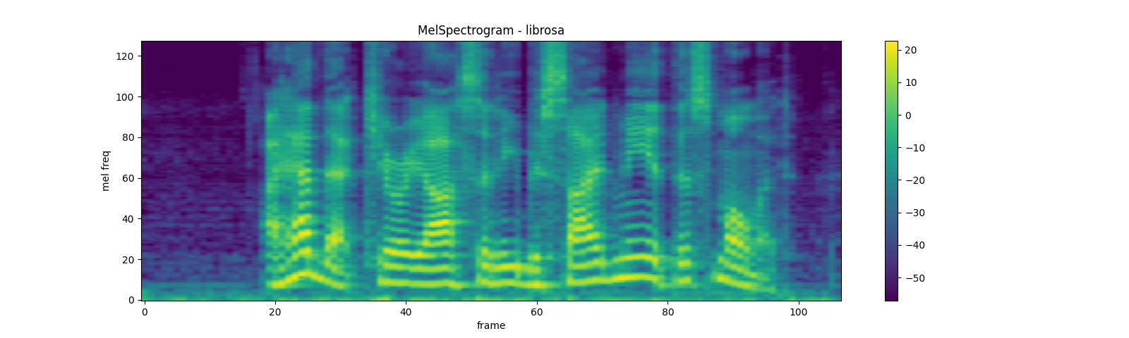
输出:

Mean Square Difference:  1.17573561997375e-10

MFCC

waveform, sample_rate = get_speech_sample()

n_fft = 2048
win_length = None
hop_length = 512
n_mels = 256
n_mfcc = 256

mfcc_transform = T.MFCC(
    sample_rate=sample_rate,
    n_mfcc=n_mfcc,
    melkwargs={
      'n_fft': n_fft,
      'n_mels': n_mels,
      'hop_length': hop_length,
      'mel_scale': 'htk',
    }
)

mfcc = mfcc_transform(waveform)

plot_spectrogram(mfcc[0])

与librosa进行比较

melspec = librosa.feature.melspectrogram(
  y=waveform.numpy()[0], sr=sample_rate, n_fft=n_fft,
  win_length=win_length, hop_length=hop_length,
  n_mels=n_mels, htk=True, norm=None)

mfcc_librosa = librosa.feature.mfcc(
  S=librosa.core.spectrum.power_to_db(melspec),
  n_mfcc=n_mfcc, dct_type=2, norm='ortho')

plot_spectrogram(mfcc_librosa)

mse = torch.square(mfcc - mfcc_librosa).mean().item()
print('Mean Square Difference: ', mse)

输出:

Mean Square Difference:  4.258112085153698e-08

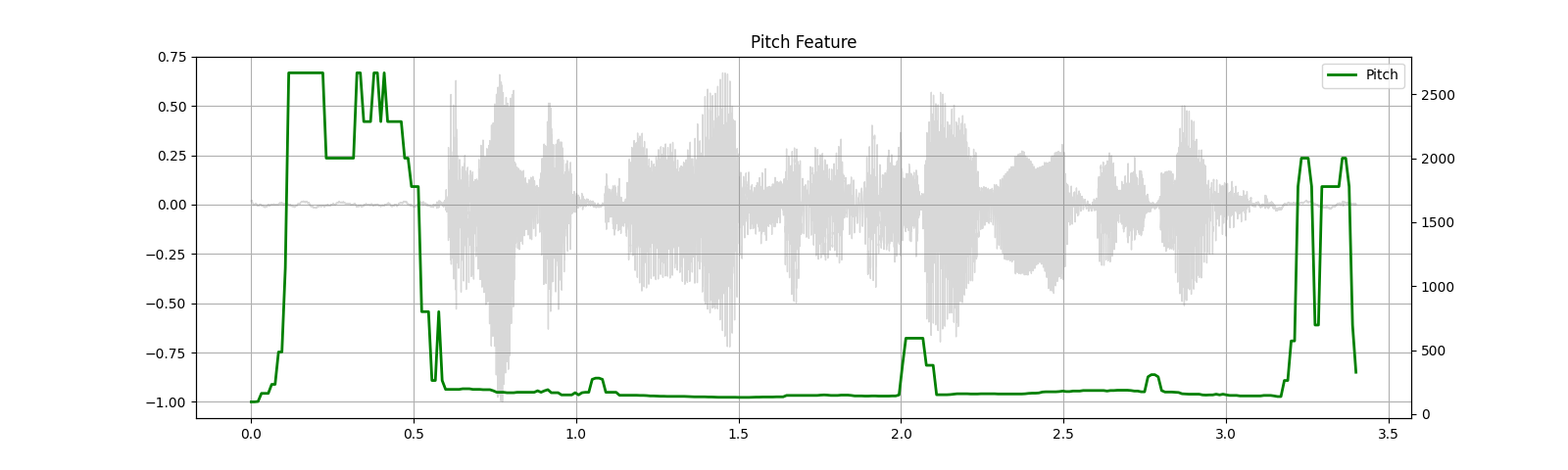
音高

waveform, sample_rate = get_speech_sample()

pitch = F.detect_pitch_frequency(waveform, sample_rate)
plot_pitch(waveform, sample_rate, pitch)
play_audio(waveform, sample_rate)

输出:

<IPython.lib.display.Audio object>

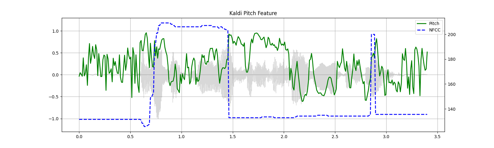
Kaldi Pitch (测试版)

Kaldi Pitch 特征 [1] 是一种为 ASR 应用调整的音高检测机制。这是 torchaudio 中的一个测试版功能，目前仅提供 functional 形式。

1. 一种为自动语音识别调整的音高提取算法

   Ghahremani, B. BabaAli, D. Povey, K. Riedhammer, J. Trmal 和 S. Khudanpur

   2014年IEEE国际声学、语音和信号处理会议（ICASSP），佛罗伦萨，2014年，第2494-2498页，doi: 10.1109/ICASSP.2014.6854049。 [摘要], [论文]

waveform, sample_rate = get_speech_sample(resample=16000)

pitch_feature = F.compute_kaldi_pitch(waveform, sample_rate)
pitch, nfcc = pitch_feature[..., 0], pitch_feature[..., 1]

plot_kaldi_pitch(waveform, sample_rate, pitch, nfcc)
play_audio(waveform, sample_rate)

输出:

<IPython.lib.display.Audio object>

特征增强

SpecAugment

SpecAugment 是一种应用于频谱图的流行增强技术。

torchaudio 实现了 TimeStrech, TimeMasking 和 FrequencyMasking.

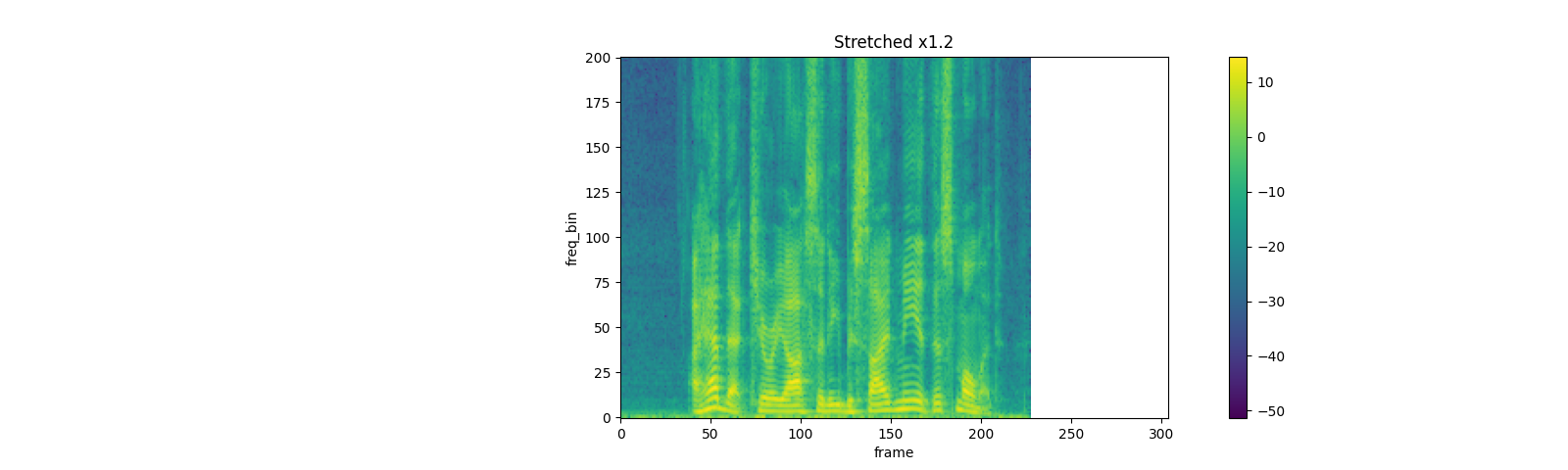
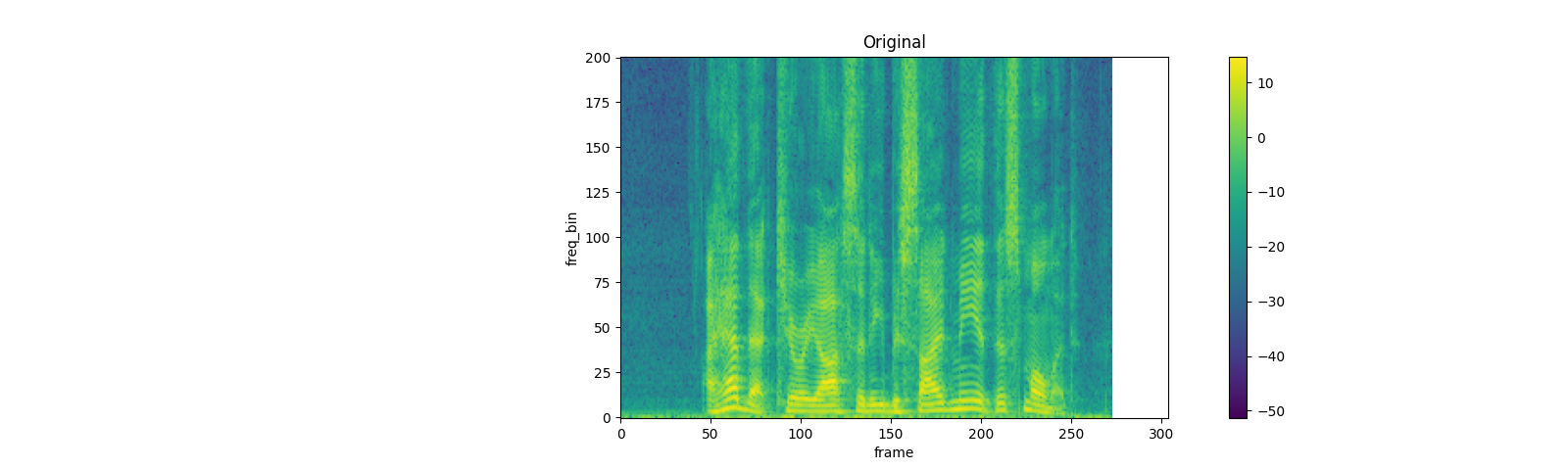
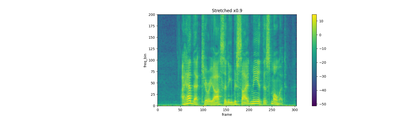
时间拉伸

spec = get_spectrogram(power=None)
strech = T.TimeStretch()

rate = 1.2
spec_ = strech(spec, rate)
plot_spectrogram(spec_[0].abs(), title=f"Stretched x{rate}", aspect='equal', xmax=304)

plot_spectrogram(spec[0].abs(), title="Original", aspect='equal', xmax=304)

rate = 0.9
spec_ = strech(spec, rate)
plot_spectrogram(spec_[0].abs(), title=f"Stretched x{rate}", aspect='equal', xmax=304)

• 
• 
• 

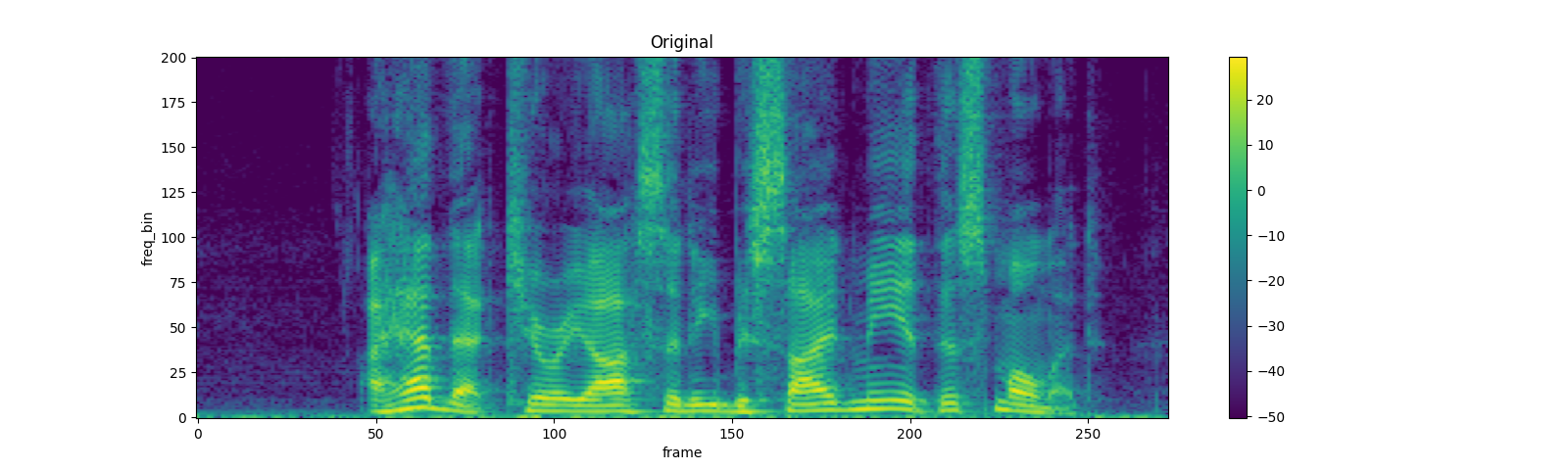
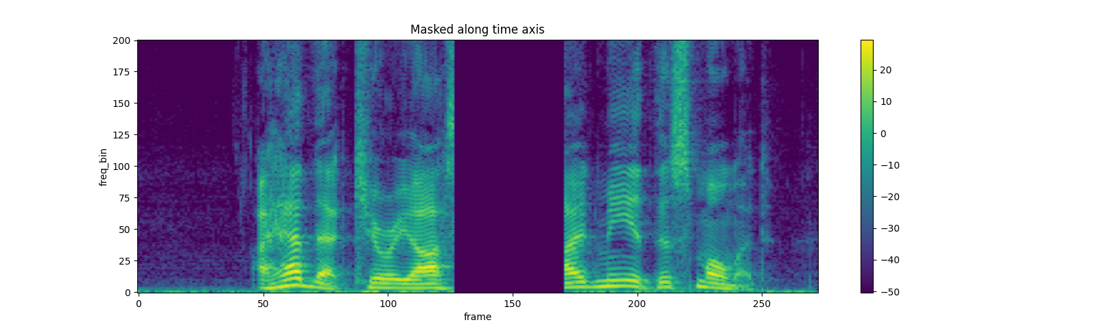
时间掩码

torch.random.manual_seed(4)

spec = get_spectrogram()
plot_spectrogram(spec[0], title="Original")

masking = T.TimeMasking(time_mask_param=80)
spec = masking(spec)

plot_spectrogram(spec[0], title="Masked along time axis")

• 
• 

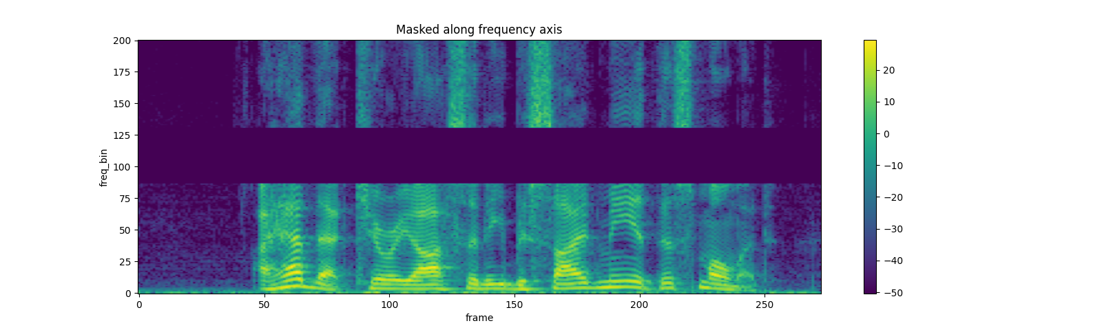
频率掩码

torch.random.manual_seed(4)

spec = get_spectrogram()
plot_spectrogram(spec[0], title="Original")

masking = T.FrequencyMasking(freq_mask_param=80)
spec = masking(spec)

plot_spectrogram(spec[0], title="Masked along frequency axis")

• 
• 

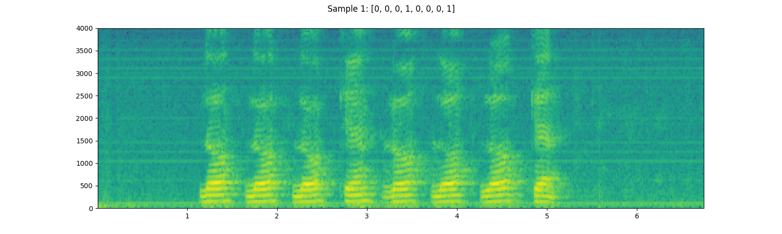
数据集

torchaudio 提供了对常见、公开可访问数据集的便捷访问。请查看官方文档以获取可用数据集的列表。

在这里，我们使用YESNO数据集，并探讨如何使用它。

YESNO_DOWNLOAD_PROCESS.join()

dataset = torchaudio.datasets.YESNO(YESNO_DATASET_PATH, download=True)

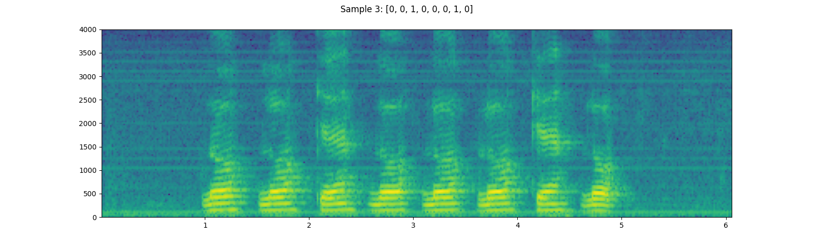
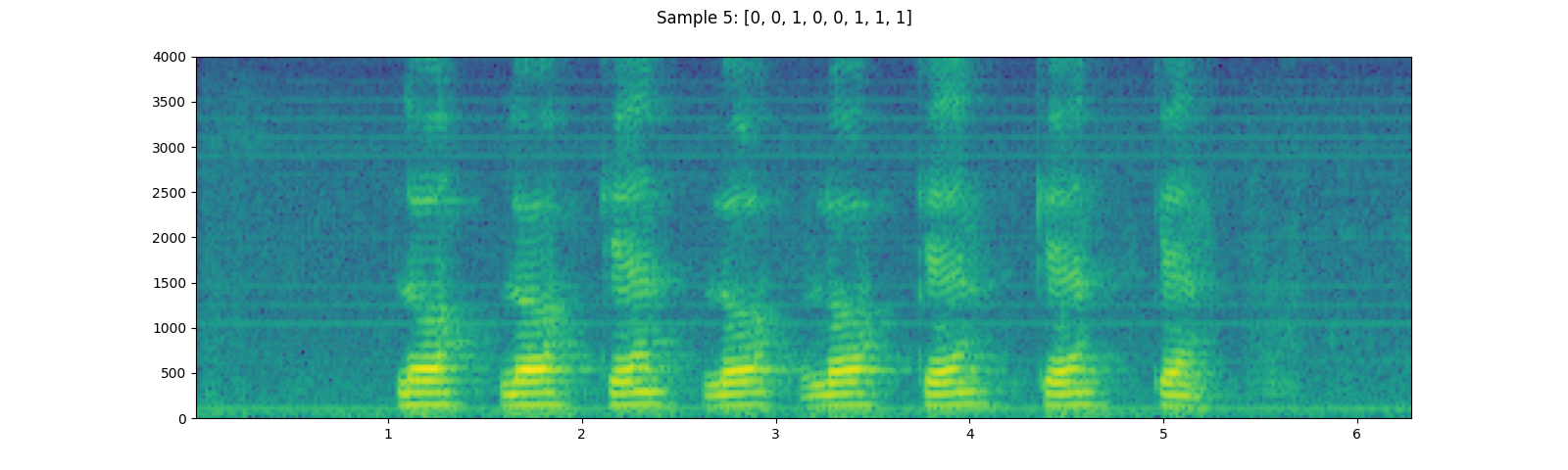
for i in [1, 3, 5]:
  waveform, sample_rate, label = dataset[i]
  plot_specgram(waveform, sample_rate, title=f"Sample {i}: {label}")
  play_audio(waveform, sample_rate)

• 
• 
• 

输出:

<IPython.lib.display.Audio object>
<IPython.lib.display.Audio object>
<IPython.lib.display.Audio object>