样本外（OOS）嵌入

Suppose we’ve embedded the nodes of a graph into Euclidean space using Adjacency Spectral Embedding (ASE) or Laplacian Spectral Embeding (LSE).

Then, suppose we gain access to new nodes not seen in the original graph. We sometimes wish to determine their latent positions without the computationally-expensive task of re-embedding an entirely new adjacency matrix.

More formally, suppose we have computed the embedding \(\hat{X} \in \textbf{R}^{n \times d}\) from some adjacency matrix \(A \in \textbf{R}^{n \times n}\).

Suppose we then obtain some new vertex with adjacency vector \(w \in \textbf{R}^n\) or new vertices with “adjacency” matrix \(W \in \textbf{R}^{m \times n}\), with \(m\) the number of new vertices. We wish to estimate the latent positions for these new vertices.

在这里，“邻接向量” \(w\) 是一个具有 \(n\) 个元素的向量，\(n\) 是样本内顶点的数量，并且在未加权的情况下，如果样本外顶点与样本内顶点 \(i\) 有边，则在第 \(i_{th}\) 位置为1。

\(W \in \textbf{R}^{m \times n}\) 是一个矩阵，每一行是一个邻接向量，用于 \(m\) 个样本外顶点。

We can obtain this estimation with ASE’s or LSE’s transform method.

Running through the Adjacency Spectral Embedding tutorial is recommended prior to this tutorial.

import numpy as np
import matplotlib.pyplot as plt
import pandas as pd
import seaborn as sns

from numpy.random import normal, poisson

from graspologic.simulations import sbm
from graspologic.embed import AdjacencySpectralEmbed as ASE
from graspologic.embed import LaplacianSpectralEmbed as LSE
from graspologic.plot import heatmap, pairplot
from graspologic.utils import remove_vertices

np.random.seed(1234)
import warnings
warnings.filterwarnings('ignore')

/home/runner/.cache/pypoetry/virtualenvs/graspologic-pkHfzCJ8-py3.10/lib/python3.10/site-packages/tqdm/auto.py:21: TqdmWarning: IProgress not found. Please update jupyter and ipywidgets. See https://ipywidgets.readthedocs.io/en/stable/user_install.html
  from .autonotebook import tqdm as notebook_tqdm

无向样本外预测

在这里，我们使用ASE嵌入了一个无向的两块随机块模型。然后，我们使用其变换方法来找到单个顶点和多个顶点的样本外预测。

我们首先生成数据。

# Generate parameters
nodes_per_community = 100
P = np.array([[0.8, 0.2],
              [0.2, 0.8]])

# Generate an undirected Stochastic Block Model (SBM)
undirected, labels_ = sbm(2*[nodes_per_community], P, return_labels=True)
labels = list(labels_)

# Grab out-of-sample vertices
oos_idx = 0
oos_labels = labels.pop(oos_idx)
A, a = remove_vertices(undirected, indices=oos_idx, return_removed=True)

# plot our SBM
heatmap(A, title=f'2-block SBM (undirected), shape {A.shape}', inner_hier_labels=labels);

嵌入 (ASE)

然后我们使用ASE生成一个嵌入，并使用其transform方法来确定我们对样本外顶点的潜在位置的最佳估计。

# Generate an embedding with ASE
ase = ASE(n_components=2)
X_hat_ase = ase.fit_transform(A)

# predicted latent positions
w_ase = ase.transform(a)
w_ase

array([ 0.69563801, -0.59472394])

绘制样本外嵌入

Here, we plot the original latent positions as well as the out-of-sample vertices. Note that the out-of-sample vertices are near their expected latent positions despite not having been run through the original embedding.

In this plot, the stars are the out-of-sample latent positions, and the dots are the in-sample latent positions.

def plot_oos(X_hat, oos_vertices, labels, oos_labels, title):
    # Plot the in-sample latent positions
    plot = pairplot(X_hat, labels=labels, title=title)

    # generate an out-of-sample dataframe
    oos_vertices = np.atleast_2d(oos_vertices)
    data = {'Type': oos_labels,
          'Dimension 1': oos_vertices[:, 0],
          'Dimension 2': oos_vertices[:, 1]}
    oos_df = pd.DataFrame(data=data)

    # update plot with out-of-sample latent positions,
    # plotting out-of-sample latent positions as stars
    plot.data = oos_df
    plot.hue_vals = oos_df["Type"]
    plot.map_offdiag(sns.scatterplot, s=500,
                     marker="*", edgecolor="black")
    plot.tight_layout()
    return plot

# Plot all latent positions
plot_oos(X_hat_ase, w_ase, labels=labels, oos_labels=[0], title="ASE Out-of-Sample Embeddings (2-block SBM)");

嵌入 (LSE)

同样，我们也可以使用拉普拉斯谱嵌入（LSE）。我们通过其变换方法生成嵌入，以确定我们对样本外顶点潜在位置的最佳估计。

# Generate an embedding with ASE
lse = LSE(n_components=2)
X_hat_lse = lse.fit_transform(A)

# predicted latent positions
w_lse = lse.transform(a)
w_lse

array([[ 0.07091005, -0.06055902]])

plot_oos(X_hat_lse, w_lse, labels=labels, oos_labels=[0], title="LSE Out-of-Sample Embeddings (2-block SBM)");

传入多个样本外顶点

你可以将一个2d numpy数组传递给transform。行是样本外的顶点，列是它们与样本内顶点的边。

# Grab out-of-sample vertices
labels = list(labels_)
oos_idx = [0, -1]
oos_labels = [labels.pop(i) for i in oos_idx]
A, a = remove_vertices(undirected, indices=oos_idx, return_removed=True)

# our out-of-sample array is m x n
print(f"a is {type(a)} with shape {a.shape}")

a is <class 'numpy.ndarray'> with shape (2, 198)

# Generate an embedding with ASE
ase = ASE(n_components=2)
X_hat_ase = ase.fit_transform(A)

# predicted latent positions
w_ase = ase.transform(a)
print(f"The out-of-sample prediction output has dimensions {w_ase.shape}\n")

# Plot all latent positions
plot_oos(X_hat_ase, w_ase, labels, oos_labels=oos_labels,
         title="ASE Out-of-Sample Embeddings (2-block SBM)");

The out-of-sample prediction output has dimensions (2, 2)

# Generate an embedding with LSE
lse = LSE(n_components=2)
X_hat_lse = lse.fit_transform(A)

# predicted latent positions
w_lse = lse.transform(a)
print(f"The out-of-sample prediction output has dimensions {w_lse.shape}\n")

# Plot all latent positions
plot_oos(X_hat_lse, w_lse, labels, oos_labels=oos_labels,
         title="LSE Out-of-Sample Embeddings (2-block SBM)");

The out-of-sample prediction output has dimensions (2, 2)

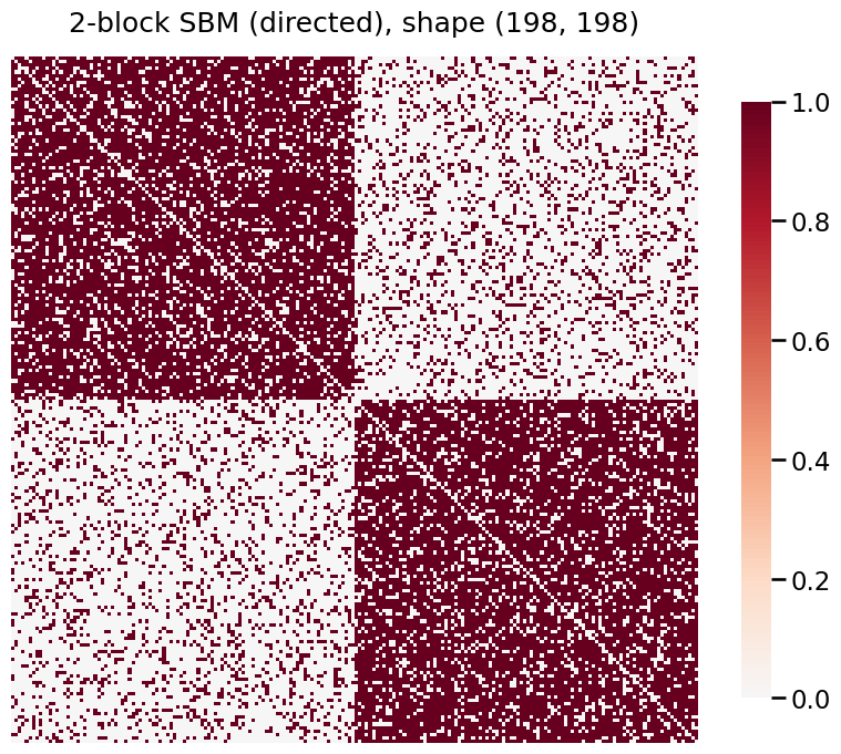
定向样本外预测

并非所有图都是无向的。当为有向图寻找样本外的潜在位置时，\(A \in \textbf{R}^{n \times n}\) 不是对称的。\(A_{i,j}\) 表示从节点 \(i\) 到节点 \(j\) 的边，而 \(A_{j, i}\) 表示从节点 \(j\) 到节点 \(i\) 的边。

To account for this, we pass a tuple (out_oos, in_oos) into the transform method. It then outputs a tuple of (out_latent_prediction, in_latent_prediction).

Here, “out” means “edges from out-of-sample vertices to in-sample vertices”

# Generate a directed SBM
directed = sbm(2*[nodes_per_community], P, directed=True)
oos_idx = [0, -1]

# a is a tuple of (out_oos, in_oos)
A, a = remove_vertices(directed, indices=oos_idx, return_removed=True)

# Plot the new adjacency matrix
heatmap(directed, title=f'2-block SBM (directed), shape {A.shape}');

# Fit our directed graph
X_hat_ase, Y_hat_ase = ase.fit_transform(A)

# predicted latent positions
w_ase = ase.transform(a)
print(f"output of `ase.transform(a)` is {type(w_ase)}", "\n")
print(f"out latent positions: \n{w_ase[0]}\n")
print(f"in latent positions: \n{w_ase[1]}")

output of `ase.transform(a)` is <class 'tuple'>

out latent positions:
[[ 0.69382889  0.56970396]
 [ 0.71045116 -0.64020639]]

in latent positions:
[[ 0.68914527  0.46260394]
 [ 0.69295841 -0.60998878]]

绘制有向ASE潜在预测

plot_oos(X_hat_ase, w_ase[0], labels, oos_labels=oos_labels, title="ASE Out Latent Predictions")
plot_oos(Y_hat_ase, w_ase[1], labels, oos_labels=oos_labels, title="ASE In Latent Predictions")

<seaborn.axisgrid.PairGrid at 0x7f7345647d00>

# Fit our directed graph
X_hat_lse, Y_hat_lse = lse.fit_transform(A)

# predicted latent positions
w_lse = lse.transform(a)
print(f"output of `ase.transform(a)` is {type(w_lse)}", "\n")
print(f"out latent positions: \n{w_lse[0]}\n")
print(f"in latent positions: \n{w_lse[1]}")

output of `ase.transform(a)` is <class 'tuple'>

out latent positions:
[[ 0.0709367   0.05849967]
 [ 0.07096437 -0.06330408]]

in latent positions:
[[ 0.07113943  0.04806502]
 [ 0.07069668 -0.0611713 ]]

绘制有向LSE潜在预测

plot_oos(X_hat_lse, w_lse[0], labels, oos_labels=oos_labels, title="LSE Out Latent Predictions")
plot_oos(Y_hat_lse, w_lse[1], labels, oos_labels=oos_labels, title="LSE In Latent Predictions")

<seaborn.axisgrid.PairGrid at 0x7f73455bc490>

加权样本外预测

加权图同样适用。在这里，我们生成一个有向加权图，并估计多个样本外顶点的潜在位置。

# Generate a weighted, directed SBM
wt = [[normal, poisson],
      [poisson, normal]]
wtargs = [[dict(loc=3, scale=1), dict(lam=5)],
          [dict(lam=5), dict(loc=3, scale=1)]]
weighted = sbm(2*[nodes_per_community], P, wt=wt, wtargs=wtargs, directed=True)

# Generate out-of-sample vertices
oos_idx = [0, -1]
A, a = remove_vertices(weighted, indices=oos_idx, return_removed=True)

# Plot our weighted, directed SBM
heatmap(A, title=f'2-block SBM (directed, weighted), shape {A.shape}')

<Axes: title={'center': '2-block SBM (directed, weighted), shape (198, 198)'}>

# Embed and transform
X_hat_ase, Y_hat_ase = ase.fit_transform(A)
w_ase = ase.transform(a)

# Plot
plot_oos(X_hat_ase, w_ase[0], labels, oos_labels=oos_labels, title="ASE Out Latent Predictions")
plot_oos(Y_hat_ase, w_ase[1],labels, oos_labels=oos_labels, title="ASE In Latent Predictions")

<seaborn.axisgrid.PairGrid at 0x7f7345a86200>

# Embed and transform
X_hat_lse, Y_hat_lse = lse.fit_transform(A)
w_lse = lse.transform(a)

# Plot
plot_oos(X_hat_lse, w_lse[0], labels, oos_labels=oos_labels, title="LSE Out Latent Predictions")
plot_oos(Y_hat_lse, w_lse[1],labels, oos_labels=oos_labels, title="LSE In Latent Predictions")

<seaborn.axisgrid.PairGrid at 0x7f7345c00b80>