先验和后验预测检查#

后验预测检查（PPCs）是验证模型的一个很好方法。其理念是使用来自后验抽样的参数从模型中生成数据。

稍微详细说明一下，可以说PPCs分析模型生成的数据与真实分布生成的数据的偏差程度。因此，您通常会想知道，比如，您的后验分布是否在近似您的基础分布。这种模型评估方法的可视化方面对于进行’基本检查’或向他人解释您的模型并获得反馈也非常有效。

先验预测检查在贝叶斯建模工作流程中也是一个关键部分。基本上，它们有两个主要好处：

它们允许您检查您是否确实将科学知识纳入到您的模型中——简而言之，它们帮助您在看到数据之前检查您的假设有多可靠。
它们可以显著帮助采样，特别是对于广义线性模型，在这些模型中，由于链接函数的缘故，结果空间和参数空间是分离的。

在这里，我们将实现一个通用的例程，从模型的观察节点中提取样本。这些模型是基础的，但它们将成为创建您自己例程的垫脚石。如果您想看到如何在更复杂的多维模型中进行先验和后验预测检查，您可以查看这个笔记本。现在，让我们开始抽样吧！

import arviz as az
import matplotlib.pyplot as plt
import numpy as np
import pymc as pm
import xarray as xr

from scipy.special import expit as logistic


print(f"Running on PyMC v{pm.__version__}")

Running on PyMC v4.4.0+207.g49b517fde.dirty

az.style.use("arviz-darkgrid")

RANDOM_SEED = 58
rng = np.random.default_rng(RANDOM_SEED)


def standardize(series):
    """标准化一个 pandas 系列"""
    return (series - series.mean()) / series.std()

让我们生成一个非常简单的线性回归模型。为了目的，我将模拟一些数据，这些数据并不来自标准正态分布（你稍后会明白原因）：

N = 100

true_a, true_b, predictor = 0.5, 3.0, rng.normal(loc=2, scale=6, size=N)
true_mu = true_a + true_b * predictor
true_sd = 2.0

outcome = rng.normal(loc=true_mu, scale=true_sd, size=N)

f"{predictor.mean():.2f}, {predictor.std():.2f}, {outcome.mean():.2f}, {outcome.std():.2f}"

'1.59, 5.69, 4.97, 17.54'

如您所见，我们的预测变量和结果变量的变化非常大——这在真实数据中是常见的。有时，采样器对此不太满意——而当您使用贝叶斯方法时，您可不想让采样器生气……所以，让我们做一些在处理真实数据时常常需要做的事情：标准化！这样，我们的预测变量和结果变量将具有均值0和标准差1，采样器会高兴得多：

predictor_scaled = standardize(predictor)
outcome_scaled = standardize(outcome)

f"{predictor_scaled.mean():.2f}, {predictor_scaled.std():.2f}, {outcome_scaled.mean():.2f}, {outcome_scaled.std():.2f}"

'0.00, 1.00, -0.00, 1.00'

现在，让我们使用传统的平坦先验来构建模型，并获取先验预测样本：

with pm.Model() as model_1:
    a = pm.Normal("a", 0.0, 10.0)
    b = pm.Normal("b", 0.0, 10.0)

    mu = a + b * predictor_scaled
    sigma = pm.Exponential("sigma", 1.0)

    pm.Normal("obs", mu=mu, sigma=sigma, observed=outcome_scaled)
    idata = pm.sample_prior_predictive(samples=50, random_seed=rng)

Sampling: [a, b, obs, sigma]

这些先验是什么意思？在纸面上总是很难判断——最好的方法是绘制它们在结果尺度上的影响，例如：

_, ax = plt.subplots()

x = xr.DataArray(np.linspace(-2, 2, 50), dims=["plot_dim"])
prior = idata.prior
y = prior["a"] + prior["b"] * x

ax.plot(x, y.stack(sample=("chain", "draw")), c="k", alpha=0.4)

ax.set_xlabel("Predictor (stdz)")
ax.set_ylabel("Mean Outcome (stdz)")
ax.set_title("Prior predictive checks -- Flat priors");

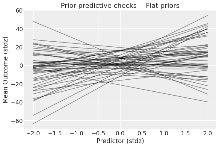
../../_images/55640e8bf2b4aa82561aefec13f5b0d35ff8e7a8dcca2b0c90cc65a81514065f.png

这些先验允许结果与预测变量之间存在极强的关系。当然，先验的选择总是取决于你的模型和数据，但看看y轴的尺度：结果可以从-40到+40个标准差（记住，数据是标准化的）。我希望你能同意，这太宽松了——我们可以做得更好！让我们使用弱信息先验，看看它们会产生什么。在实际案例研究中，这就是你将科学知识融入模型的部分：

with pm.Model() as model_1:
    a = pm.Normal("a", 0.0, 0.5)
    b = pm.Normal("b", 0.0, 1.0)

    mu = a + b * predictor_scaled
    sigma = pm.Exponential("sigma", 1.0)

    pm.Normal("obs", mu=mu, sigma=sigma, observed=outcome_scaled)
    idata = pm.sample_prior_predictive(samples=50, random_seed=rng)

Sampling: [a, b, obs, sigma]

_, ax = plt.subplots()

x = xr.DataArray(np.linspace(-2, 2, 50), dims=["plot_dim"])
prior = idata.prior
y = prior["a"] + prior["b"] * x

ax.plot(x, y.stack(sample=("chain", "draw")), c="k", alpha=0.4)

ax.set_xlabel("Predictor (stdz)")
ax.set_ylabel("Mean Outcome (stdz)")
ax.set_title("Prior predictive checks -- Weakly regularizing priors");

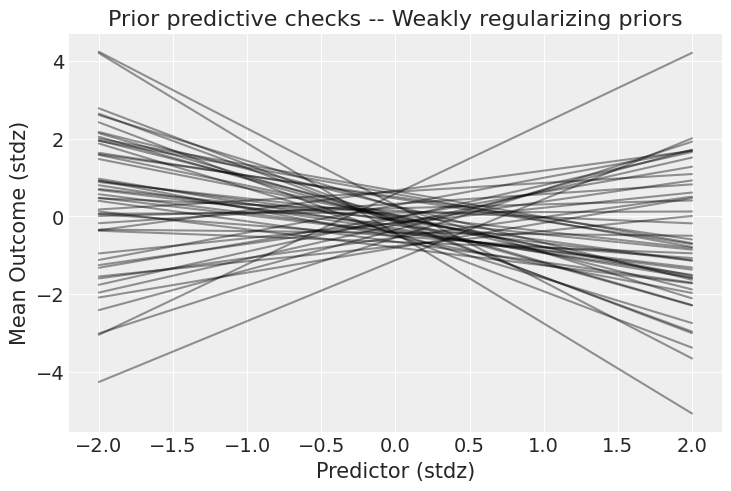
../../_images/cbc230a3b9c32c4d010baf2de311d7e37dd549bd6bbee166aa9bf020c48e992a.png

好得多！虽然仍然有非常强的关系，但至少现在结果仍然在可能的范围内。现在，是时候庆祝了——当然，如果你所说的“庆祝”是指“运行模型”。

with model_1:
    idata.extend(pm.sample(1000, tune=2000, random_seed=rng))

az.plot_trace(idata);

Auto-assigning NUTS sampler...
Initializing NUTS using jitter+adapt_diag...
Multiprocess sampling (3 chains in 3 jobs)
NUTS: [a, b, sigma]

100.00% [9000/9000 00:07<00:00 Sampling 3 chains, 0 divergences]

Sampling 3 chains for 2_000 tune and 1_000 draw iterations (6_000 + 3_000 draws total) took 37 seconds.

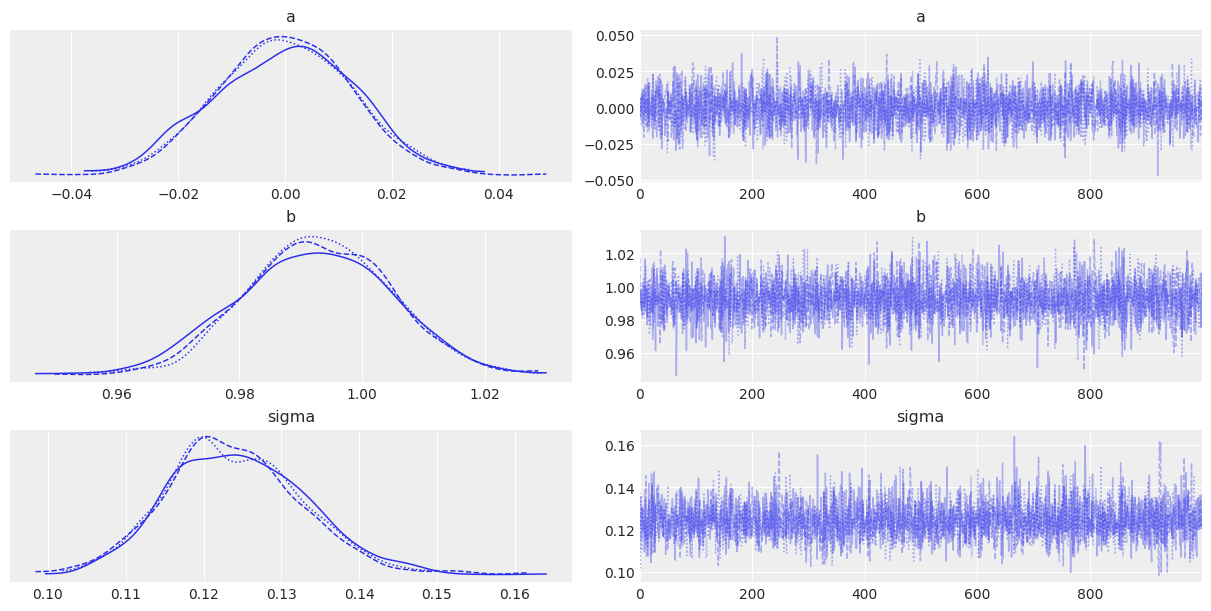
../../_images/dff5ffc3adba18eee70cc2f3c19427475b4b289105ee834f84ce0d40ea9c331c.png

一切运行顺利，但在分析跟踪图或表摘要时，理解参数值的含义常常很困难——尤其是在这里，因为参数存在于标准化空间中。理解模型的一个有用方法是……你猜对了：后验预测检查！我们将使用PyMC的专用函数从后验中抽样数据。该函数将随机从跟踪中抽取4000个参数样本。然后，对于每个样本，它将从由该样本中的mu和sigma值指定的正态分布中抽取100个随机数：

with model_1:
    pm.sample_posterior_predictive(idata, extend_inferencedata=True, random_seed=rng)

Sampling: [obs]

100.00% [3000/3000 00:00<00:00]

现在，idata中的posterior_predictive组包含4000个生成的数据集（每个数据集包含100个样本），每个数据集使用的参数设置来自后验分布的不同值：

一种常见的可视化方法是查看模型是否能够再现真实数据中观察到的模式。ArviZ 具有一个非常实用的函数，可以直接实现这一点：

az.plot_ppc(idata, num_pp_samples=100);

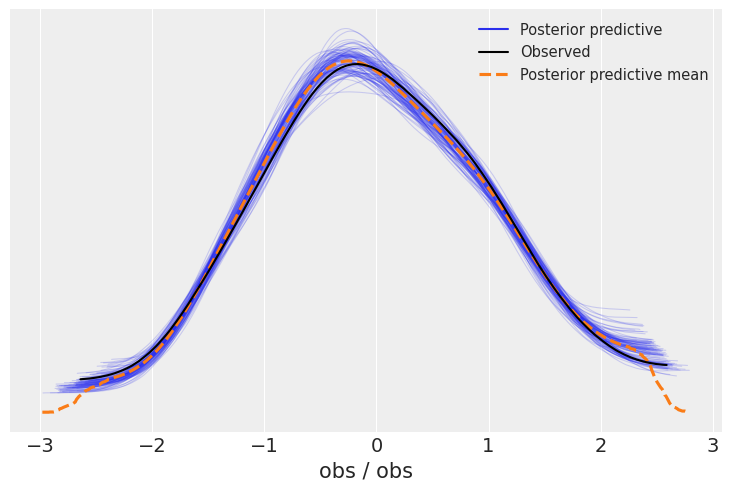
../../_images/74fa95e49111941074eb7da4d5fdd2c7875faf3ca28dfe851640639f7944b662.png

看起来模型在逆推数据方面表现得相当不错。除了这个通用函数，制作一个针对您的使用案例的图表总是很有趣。在这里，绘制预测变量和结果之间的预测关系将非常有趣。现在我们已经采样了后验预测样本，这一点非常简单——我们只需要将参数通过模型传递即可：

post = idata.posterior
mu_pp = post["a"] + post["b"] * xr.DataArray(predictor_scaled, dims=["obs_id"])

_, ax = plt.subplots()

ax.plot(
    predictor_scaled, mu_pp.mean(("chain", "draw")), label="Mean outcome", color="C1", alpha=0.6
)
ax.scatter(predictor_scaled, idata.observed_data["obs"])
az.plot_hdi(predictor_scaled, idata.posterior_predictive["obs"])

ax.set_xlabel("Predictor (stdz)")
ax.set_ylabel("Outcome (stdz)");

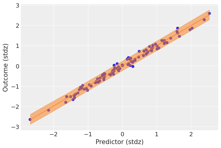
../../_images/1721dbb905460007625500abef58c770e9dc00b3f445cc7b3c528c0167e1d3dd.png

我们有很多数据，因此结果均值周围的不确定性相对较小；但结果的总体不确定性似乎与观察到的数据相符。

PPC与其他模型评估方法的比较#

在Edward文档中有一个很好的介绍：

PPC是修正模型的优秀工具，在研究模型与数据的拟合程度时，可以简化或扩展当前模型。它们的灵感来源于先验检查和经典假设检验，基于模型应在大样本评估的频率观点下受到批评的哲学。

PPC也可以应用于假设检验、模型比较、模型选择和模型平均等任务。需要注意的是，尽管它们可以作为贝叶斯假设检验的一种形式，但通常不建议进行假设检验：从单个测试进行二元决策并不是像人们想象的那样常见的用例。我们建议执行多次PPC，以全面了解模型拟合情况。

预测#

相同的模式可以用于预测。在这里，我们构建一个逻辑回归模型：

N = 400
true_intercept = 0.2
true_slope = 1.0
predictors = rng.normal(size=N)
true_p = logistic(true_intercept + true_slope * predictors)

outcomes = rng.binomial(1, true_p)
outcomes[:10]

array([1, 1, 1, 1, 0, 1, 0, 0, 1, 1], dtype=int64)

with pm.Model() as model_2:
    betas = pm.Normal("betas", mu=0.0, sigma=np.array([0.5, 1.0]), shape=2)

    # 将预测变量设置为共享变量以更改PPCs的设置：
    pred = pm.MutableData("pred", predictors, dims="obs_id")
    p = pm.Deterministic("p", pm.math.invlogit(betas[0] + betas[1] * pred), dims="obs_id")

    outcome = pm.Bernoulli("outcome", p=p, observed=outcomes, dims="obs_id")

    idata_2 = pm.sample(1000, tune=2000, return_inferencedata=True, random_seed=rng)
az.summary(idata_2, var_names=["betas"], round_to=2)

Auto-assigning NUTS sampler...
Initializing NUTS using jitter+adapt_diag...
Multiprocess sampling (3 chains in 3 jobs)
NUTS: [betas]

100.00% [9000/9000 00:07<00:00 Sampling 3 chains, 0 divergences]

Sampling 3 chains for 2_000 tune and 1_000 draw iterations (6_000 + 3_000 draws total) took 37 seconds.

	mean	sd	hdi_3%	hdi_97%	mcse_mean	mcse_sd	ess_bulk	ess_tail	r_hat
betas[0]	0.23	0.11	0.03	0.43	0.0	0.0	2175.39	2203.68	1.0
betas[1]	1.04	0.14	0.76	1.29	0.0	0.0	2635.17	2032.97	1.0

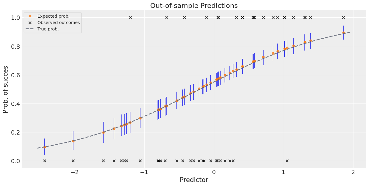
现在，让我们模拟一些样本外数据，看看模型如何进行预测。我们将新的预测变量提供给模型，然后它将根据在训练阶段学到的内容告诉我们它认为的结果。接着，我们将把模型的预测与真实的样本外结果进行比较。

predictors_out_of_sample = rng.normal(size=50)
outcomes_out_of_sample = rng.binomial(
    1, logistic(true_intercept + true_slope * predictors_out_of_sample)
)

with model_2:
    # 更新预测变量的值：
    pm.set_data({"pred": predictors_out_of_sample})
    # 使用更新后的数值预测结果和概率：
    idata_2 = pm.sample_posterior_predictive(
        idata_2,
        var_names=["p"],
        return_inferencedata=True,
        predictions=True,
        extend_inferencedata=True,
        random_seed=rng,
    )

Sampling: []

100.00% [3000/3000 00:00<00:00]

平均预测值加误差条以给出预测的不确定性感#

请注意，由于我们处理的是完整的后验分布，因此我们的预测中也自然而然地获得了不确定性。

_, ax = plt.subplots(figsize=(12, 6))

preds_out_of_sample = idata_2.predictions_constant_data.sortby("pred")["pred"]
model_preds = idata_2.predictions.sortby(preds_out_of_sample)

# 对估计的不确定性：
ax.vlines(
    preds_out_of_sample,
    *az.hdi(model_preds)["p"].transpose("hdi", ...),
    alpha=0.8,
)
# 预期成功概率：
ax.plot(
    preds_out_of_sample,
    model_preds["p"].mean(("chain", "draw")),
    "o",
    ms=5,
    color="C1",
    alpha=0.8,
    label="Expected prob.",
)

# 实际结果：
ax.scatter(
    x=predictors_out_of_sample,
    y=outcomes_out_of_sample,
    marker="x",
    color="k",
    alpha=0.8,
    label="Observed outcomes",
)
# 真实概率：
x = np.linspace(predictors_out_of_sample.min() - 0.1, predictors_out_of_sample.max() + 0.1)
ax.plot(
    x,
    logistic(true_intercept + true_slope * x),
    lw=2,
    ls="--",
    color="#565C6C",
    alpha=0.8,
    label="True prob.",
)

ax.set_xlabel("Predictor")
ax.set_ylabel("Prob. of success")
ax.set_title("Out-of-sample Predictions")
ax.legend(fontsize=10, frameon=True, framealpha=0.5);

../../_images/5c4af8eeb312e7c8e924abcd409809b2a6ee170f26817ff6fbe16640acdea433.png

%load_ext watermark
%watermark -n -u -v -iv -w -p pytensor

Last updated: Tue Dec 06 2022

Python implementation: CPython
Python version       : 3.11.0
IPython version      : 8.7.0

pytensor: 2.8.10

matplotlib: 3.6.2
xarray    : 2022.12.0
pymc      : 4.4.0+207.g7c3068a1c
numpy     : 1.23.4
arviz     : 0.14.0

Watermark: 2.3.1