import arviz as az
import matplotlib.pyplot as plt
import numpy as np
import pymc as pm

print(f"Running on PyMC v{pm.__version__}")
Running on PyMC v4.4.0+213.g85ca9123f.dirty
az.style.use("arviz-darkgrid")
模型比较#
为了演示在PyMC中使用模型比较标准,我们实现了Gelman等人(2003)第5.5节中的8所学校示例,该示例试图推断来自8所学校的学生在SAT成绩上接受辅导的效果。下面,我们拟合一个合并模型,假设所有学校都具有一个固定效应,以及一个分层模型,允许存在一个随机效应,该效应部分汇总数据。
数据包括在8所学校中观察到的治疗效果(y)及其相关的标准差(sigma)。
y = np.array([28, 8, -3, 7, -1, 1, 18, 12])
sigma = np.array([15, 10, 16, 11, 9, 11, 10, 18])
J = len(y)
合成模型#
with pm.Model() as pooled:
    # 潜在的合并效应量
    mu = pm.Normal("mu", 0, sigma=1e6)

    obs = pm.Normal("obs", mu, sigma=sigma, observed=y)

    trace_p = pm.sample(2000)
Auto-assigning NUTS sampler...
Initializing NUTS using jitter+adapt_diag...
Multiprocess sampling (4 chains in 4 jobs)
NUTS: [mu]
Sampling 4 chains for 1_000 tune and 2_000 draw iterations (4_000 + 8_000 draws total) took 3 seconds.
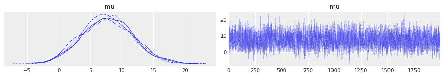
az.plot_trace(trace_p);
层次模型#
with pm.Model() as hierarchical:
    eta = pm.Normal("eta", 0, 1, shape=J)
    # 分层均值和标准差
    mu = pm.Normal("mu", 0, sigma=10)
    tau = pm.HalfNormal("tau", 10)

    # 随机效应的非中心参数化
    theta = pm.Deterministic("theta", mu + tau * eta)

    obs = pm.Normal("obs", theta, sigma=sigma, observed=y)

    trace_h = pm.sample(2000, target_accept=0.9)
Auto-assigning NUTS sampler...
Initializing NUTS using jitter+adapt_diag...
Multiprocess sampling (4 chains in 4 jobs)
NUTS: [eta, mu, tau]
Sampling 4 chains for 1_000 tune and 2_000 draw iterations (4_000 + 8_000 draws total) took 10 seconds.
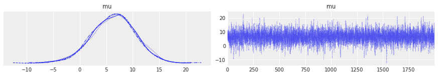
az.plot_trace(trace_h, var_names="mu");
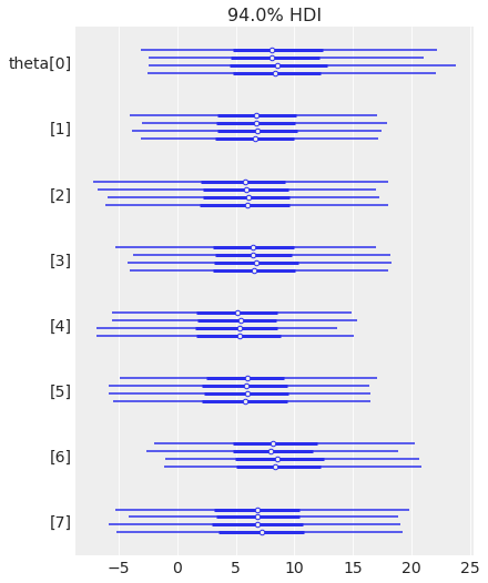
az.plot_forest(trace_h, var_names="theta");
留一法交叉验证 (LOO)#
留一法交叉验证是对样本外预测适配度的估计。在交叉验证中,数据被反复划分为训练集和验证集,迭代地用前者拟合模型,并用验证数据评估拟合效果。Vehtari等人(2016)提出了一种根据MCMC样本高效计算LOO的方法(无需重新拟合数据)。该近似基于重要性抽样。重要性权重通过一种称为Pareto平滑重要性抽样(PSIS)的方法进行稳定化。
广泛适用的信息准则 (WAIC)#
WAIC(Watanabe 2010)是一个完全贝叶斯的准则,用于估计样本外期望,使用计算出的对数逐点后验预测密度(LPPD)并对有效参数数量进行校正以调整过拟合。
默认情况下,ArviZ使用LOO,但也提供WAIC。
模型对数似然#
为了计算LOO和WAIC,ArviZ需要访问每个后验样本的模型逐元素对数似然。我们可以通过compute_log_likelihood()将其添加。或者,我们可以将idata_kwargs={"log_likelihood": True}传递给sample(),以便在采样结束时自动计算。
with pooled:
    pm.compute_log_likelihood(trace_p)
pooled_loo = az.loo(trace_p)

pooled_loo
Computed from 8000 posterior samples and 8 observations log-likelihood matrix.

         Estimate       SE
elpd_loo   -30.55     1.10
p_loo        0.67        -
------

Pareto k diagnostic values:
                         Count   Pct.
(-Inf, 0.5]   (good)        8  100.0%
 (0.5, 0.7]   (ok)          0    0.0%
   (0.7, 1]   (bad)         0    0.0%
   (1, Inf)   (very bad)    0    0.0%
with hierarchical:
    pm.compute_log_likelihood(trace_h)
hierarchical_loo = az.loo(trace_h)

hierarchical_loo
/home/ricardo/miniconda3/envs/pymc/lib/python3.10/site-packages/arviz/stats/stats.py:802: UserWarning: Estimated shape parameter of Pareto distribution is greater than 0.7 for one or more samples. You should consider using a more robust model, this is because importance sampling is less likely to work well if the marginal posterior and LOO posterior are very different. This is more likely to happen with a non-robust model and highly influential observations.
  warnings.warn(
Computed from 8000 posterior samples and 8 observations log-likelihood matrix.

         Estimate       SE
elpd_loo   -30.82     1.07
p_loo        1.17        -

There has been a warning during the calculation. Please check the results.
------

Pareto k diagnostic values:
                         Count   Pct.
(-Inf, 0.5]   (good)        1   12.5%
 (0.5, 0.7]   (ok)          6   75.0%
   (0.7, 1]   (bad)         1   12.5%
   (1, Inf)   (very bad)    0    0.0%
ArviZ包含两个便利函数以帮助比较不同模型的LOO。第一个函数是compare,它从一组痕迹和模型中计算LOO(或WAIC)并返回一个DataFrame。
df_comp_loo = az.compare({"hierarchical": trace_h, "pooled": trace_p})
df_comp_loo
/home/ricardo/miniconda3/envs/pymc/lib/python3.10/site-packages/arviz/stats/stats.py:802: UserWarning: Estimated shape parameter of Pareto distribution is greater than 0.7 for one or more samples. You should consider using a more robust model, this is because importance sampling is less likely to work well if the marginal posterior and LOO posterior are very different. This is more likely to happen with a non-robust model and highly influential observations.
  warnings.warn(
| rank | elpd_loo | p_loo | elpd_diff | weight | se | dse | warning | scale | |
|---|---|---|---|---|---|---|---|---|---|
| pooled | 0 | -30.554172 | 0.670458 | 0.000000 | 1.0 | 1.102705 | 0.000000 | False | log |
| hierarchical | 1 | -30.821814 | 1.167435 | 0.267641 | 0.0 | 1.070727 | 0.239078 | True | log |
我们有很多列,让我们逐一查看它们的含义:
索引是模型的名称,这些名称取自传递给
compare(.)的字典的键。rank,模型的排名,从0(最佳模型)开始,到模型数量。
loo,LOO(或WAIC)的值。数据框始终按最佳LOO/WAIC到最差LOO/WAIC的顺序排序。
p_loo,惩罚项的值。我们可以粗略地将该值视为估计的有效参数数量(但不要太认真对待)。
d_loo,排名最高的模型的LOO/WAIC值与每个模型的LOO/WAIC值之间的相对差异。因此,我们总是会得到第一个模型的值为0。
weight,分配给每个模型的权重。这些权重可以放松地解释为给定数据情况下每个模型为真的概率(在比较的模型中)。
se,LOO/WAIC计算的标准误差。标准误差可以帮助评估LOO/WAIC估计的不确定性。默认情况下,这些误差是通过堆叠计算得出的。
dse,两个LOO/WAIC值之间差异的标准误差。我们可以像计算每个LOO/WAIC值的标准误差一样计算两个LOO/WAIC值之间差异的标准误差。注意,这两个量不一定相同,原因是对于各个模型的LOO/WAIC的不确定性是相关的。对于排名最高的模型,该值始终为0。
warning,如果为
True,则LOO/WAIC的计算可能不可靠。loo_scale,报告值的刻度。默认是前面提到的对数刻度。其他选项是偏差 – 这是对数分数乘以 -2(这会反转顺序:较低的LOO/WAIC将更好)– 和负对数 – 这是对数分数乘以 -1(与偏差刻度一样,较低的值更好)。
第二个便利函数接受compare的输出,并生成一个总结图,样式与Richard McElreath的书《统计重思考》(Statistical Rethinking)中使用的图相似(还可以参考这个移植版本,将书中的示例转换为PyMC)。
az.plot_compare(df_comp_loo, insample_dev=False);
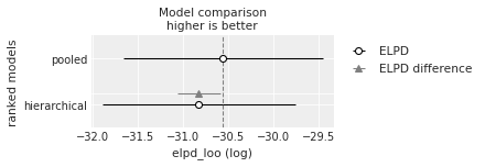
空心圆表示LOO的值,相关的黑色误差条表示LOO的标准差值。
最高LOO值,即最佳估计模型的值,也用一条垂直的虚线灰色线表示,以便与其他LOO值进行比较。
除了排名最高的模型外,我们还用一个三角形表示该模型与排名最高模型之间WAIC的差值,并用灰色误差条表示排名最高的WAIC与每个模型的WAIC之间差值的标准误差。
解释#
尽管我们可能预期分层模型会优于完全合并模型,但在这种情况下,这两种模型几乎没有区别,因为这两种模型给出的信息标准值非常相似。当我们考虑LOO和WAIC的不确定性(以标准误差表示)时,这一点更加明显。
参考文献#
Gelman, A., Hwang, J., & Vehtari, A. (2014). 理解贝叶斯模型的预测信息标准。统计与计算, 24(6), 997–1016.
Vehtari, A, Gelman, A, Gabry, J. (2016). 使用留一法交叉验证和WAIC进行实用的贝叶斯模型评估。统计与计算
%load_ext watermark

%watermark -n -u -v -iv -w -p xarray,pytensor
Last updated: Thu Dec 08 2022

Python implementation: CPython
Python version       : 3.10.8
IPython version      : 8.3.0

xarray  : 2022.6.0
pytensor: 2.8.10

pymc      : 4.4.0+213.g85ca9123f.dirty
arviz     : 0.13.0
numpy     : 1.22.3
matplotlib: 3.5.2

Watermark: 2.3.1