pyts.image.递归图
-
class
pyts.image.RecurrencePlot(dimension=1, time_delay=1, threshold=None, percentage=10, flatten=False)[来源]¶ 递归图。
递归图是一种图像,用于表示从原始时间序列中提取的轨迹之间的距离。
Parameters: - dimension : int or float (default = 1)
轨迹的维度。如果是浮点数,它表示每个时间序列大小的百分比,必须在0到1之间。
- time_delay : int or float (default = 1)
轨迹中两个连续点之间的时间间隔。如果是浮点数,它表示每个时间序列大小的百分比,必须在0到1之间。
- threshold : float, ‘point’, ‘distance’ or None (default = None)
最小距离的阈值。如果为None,则递归图不会被二值化。如果为'point',则计算阈值使得percentage百分比的点小于该阈值。如果为'distance',则计算阈值作为最大距离的percentage百分比。
- percentage : int or float (default = 10)
如果
threshold='point'则为黑点的百分比,如果threshold='distance'则为最大距离的百分比阈值。 如果threshold是浮点数或None则忽略。- flatten : bool (default = False)
如果为True,图像将被展平为一维。
注意事项
给定一个时间序列
 ,提取的轨迹是
其中
 是轨迹的
是轨迹的 dimension维度, 是 time_delay时间延迟。递归图(记作)表示轨迹之间的成对距离
其中
 是赫维赛德函数, 是
 threshold。参考文献
[1] J.-P Eckmann, S. Oliffson Kamphorst 和 D Ruelle,《动力系统的递归图》。欧洲物理快报(1987)。 示例
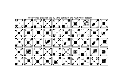
>>> from pyts.datasets import load_gunpoint
>>> from pyts.image import RecurrencePlot
>>> X, _, _, _ = load_gunpoint(return_X_y=True)
>>> transformer = RecurrencePlot()
>>> X_new = transformer.transform(X)
>>> X_new.shape
(50, 150, 150)
方法
__init__([dimension, time_delay, threshold, …])Initialize self. fit([X, y])Pass. fit_transform(X[, y])Fit to data, then transform it. get_params([deep])Get parameters for this estimator. set_params(**params)Set the parameters of this estimator. transform(X)Transform each time series into a recurrence plot. -
__init__(dimension=1, time_delay=1, threshold=None, percentage=10, flatten=False)[来源]¶ 初始化自身。查看 help(type(self)) 获取准确的签名信息。
-
fit_transform(X, y=None, **fit_params)¶ 拟合数据,然后进行转换。
使用可选参数fit_params将转换器适配到X和y,并返回转换后的X版本。
参数: - X : array-like, shape = (n_samples, n_timestamps)
单变量时间序列。
- y : None or array-like, shape = (n_samples,) (default = None)
目标值(无监督转换时为None)。
- **fit_params : dict
额外的拟合参数。
返回值: - X_new : array
转换后的数组。
-
get_params(deep=True)¶ 获取此估计器的参数。
参数: - deep : bool, default=True
如果为True,将返回此估计器及其包含的子估计器的参数。
返回值: - params : dict
参数名称映射到对应的值。