验证

由于除了实验数据外，真实值不可用，因此无法以与常规机器学习预测相同的方式验证治疗效果。在这里，我们重点关注在潜在结果无混淆性和基于我们可用的特征集处理状态的假设下的内部验证方法。

使用多个估计值进行验证

我们可以通过将估计值与其他方法进行比较，检查不同层次和群体之间估计值的一致性来验证该方法。

元算法的模型鲁棒性

在元算法中，我们可以通过比较来自不同底层机器学习算法的估计值来评估用户层面治疗效果估计的质量。我们将报告均方误差（MSE）、覆盖率（重叠95%置信区间）和提升曲线。此外，我们可以在一个队列内分割样本，并比较样本外评分和样本内评分的结果。

用户级别/细分级别/群组级别一致性

我们还可以通过进行T检验来评估用户级别/细分级别/队列级别的估计一致性。

队列之间的稳定性

治疗效果可能因群体而异，但不应过于波动。对于给定的群体，我们将比较模型拟合生成的分数与由其自身模型生成的分数。

使用合成数据集进行验证

我们可以通过模拟来测试该方法，其中我们生成的数据在结果、治疗和一些混杂变量之间具有已知的因果和非因果联系。

我们基于[19]实现了以下几组合成数据生成机制：

机制1

This generates a complex outcome regression model with easy treatment effect with input variables \(X_i \sim Unif(0, 1)^d\).

The treatment flag is a binomial variable, whose d.g.p. is:

\(P(W_i = 1 | X_i) = trim_{0.1}(sin(\pi X_{i1} X_{i2})\)

With :

\(trim_\eta(x)=\max (\eta,\min (x,1-\eta))\)

The outcome variable is:

\(y_i = sin(\pi X_{i1} X_{i2}) + 2(X_{i3} - 0.5)^2 + X_{i4} + 0.5 X_{i5} + (W_i - 0.5)(X_{i1} + X_{i2})/ 2 + \epsilon_i\)

机制2

This simulates a randomized trial. The input variables are generated by \(X_i \sim N(0, I_{d\times d})\)

The treatment flag is generated by a fair coin flip:

\(P(W_i = 1|X_i) = 0.5\)

The outcome variable is

\(y_i = max(X_{i1} + X_{i2}, X_{i3}, 0) + max(X_{i4} + X_{i5}, 0) + (W_i - 0.5)(X_{i1} + \log(1 + e^{X_{i2}}))\)

机制3

This one has an easy propensity score but a difficult control outcome. The input variables follow \(X_i \sim N(0, I_{d\times d})\)

The treatment flag is a binomial variable, whose d.g.p is:

\(P(W_i = 1 | X_i) = \frac{1}{1+\exp{X_{i2} + X_{i3}}}\)

The outcome variable is:

\(y_i = 2\log(1 + e^{X_{i1} + X_{i2} + X_{i3}}) + (W_i - 0.5)\)

机制4

This contains an unrelated treatment arm and control arm, with input data generated by \(X_i \sim N(0, I_{d\times d})\).

The treatment flag is a binomial variable whose d.g.p. is:

\(P(W_i = 1 | X_i) = \frac{1}{1+\exp{-X_{i1}} + \exp{-X_{i2}}}\)

The outcome variable is:

\(y_i = \frac{1}{2}\big(max(X_{i1} + X_{i2} + X_{i3}, 0) + max(X_{i4} + X_{i5}, 0)\big) + (W_i - 0.5)(max(X_{i1} + X_{i2} + X_{i3}, 0) - max(X_{i4}, X_{i5}, 0))\)

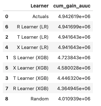
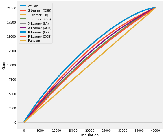
使用提升曲线进行验证 (AUUC)

我们可以通过评估和比较AUUC（提升曲线下面积）的提升增益来验证估计，它计算累积增益。更多详情请参见meta_learners_with_synthetic_data.ipynb示例笔记本。

from causalml.dataset import *
from causalml.metrics import *
# Single simulation
train_preds, valid_preds = get_synthetic_preds_holdout(simulate_nuisance_and_easy_treatment,
                                                       n=50000,
                                                       valid_size=0.2)
# Cumulative Gain AUUC values for a Single Simulation of Validaiton Data
get_synthetic_auuc(valid_preds)

对于处理偏斜的数据，有时使用目标最大似然估计（TMLE）用于ATE来生成AUUC曲线进行验证是有利的，因为TMLE提供了更准确的ATE估计。请参阅validation_with_tmle.ipynb示例笔记本以获取详细信息。

敏感性分析验证

敏感性分析旨在检查无混淆假设的稳健性。如果存在隐藏偏差（未观察到的混淆因素），它通过检查平均处理效应估计来确定需要多严重才能改变结论。

我们实施了以下方法来进行敏感性分析：

安慰剂治疗

Replace treatment with a random variable.

无关的额外混杂因素

Add a random common cause variable.

子集验证

Remove a random subset of the data.

随机替换

Random replace a covariate with an irrelevant variable.

选择偏差

Blackwell(2013) <https://www.mattblackwell.org/files/papers/sens.pdf> introduced an approach to sensitivity analysis for causal effects that directly models confounding or selection bias.

One Sided Confounding Function: here as the name implies, this function can detect sensitivity to one-sided selection bias, but it would fail to detect other deviations from ignobility. That is, it can only determine the bias resulting from the treatment group being on average better off or the control group being on average better off.

Alignment Confounding Function: this type of bias is likely to occur when units select into treatment and control based on their predicted treatment effects

The sensitivity analysis is rigid in this way because the confounding function is not identified from the data, so that the causal model in the last section is only identified conditional on a specific choice of that function. The goal of the sensitivity analysis is not to choose the “correct” confounding function, since we have no way of evaluating this correctness. By its very nature, unmeasured confounding is unmeasured. Rather, the goal is to identify plausible deviations from ignobility and test sensitivity to those deviations. The main harm that results from the incorrect specification of the confounding function is that hidden biases remain hidden.