![]()
时间序列分类、回归、聚类及其他#
本笔记本概述#
时间序列分类、回归、聚类的介绍
sktime数据格式用于“时间序列面板” = 时间序列的集合TSC、TSR、TSCl 的基本小插图
高级案例 - 管道、集成、调优
处理 时间序列集合 = “面板数据”
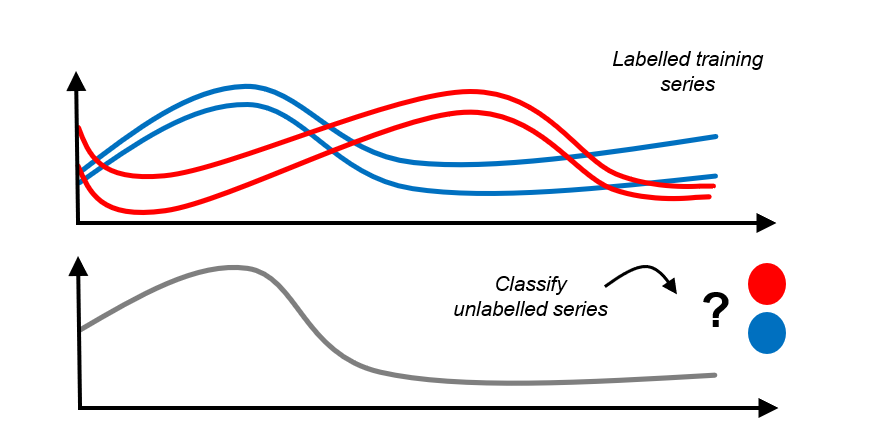
分类 = 尝试在基于时间序列/类别示例训练后,为每个时间序列分配一个 类别。
示例:随时间变化的每日能耗曲线 - 预测季节,例如,冬季/夏季,或消费者类型
回归 = 在基于时间序列/类别示例训练后,尝试为每个时间序列分配一个 类别。
示例:化学反应器的温度/压力/时间分布 - 预测总纯度(1的分数)
聚类 = 将不同的时间序列放入少量相似性桶中
示例:服务级别协议 (SLA) 违规 - 将收集的面板数据分组以识别 SLA 失败的常见原因
时间序列分类:
[1]:
import numpy as np
import pandas as pd

# Increase display width
pd.set_option("display.width", 1000)
2.1 面板数据 - sktime 数据格式#
Panel 是一种抽象数据类型,其中值被观察为:
实例,例如,患者variable,例如,患者的血压、体温time/index,例如,2023年1月12日(通常但不一定是时间索引!)
一个值 X 是:“患者 ‘A’ 在 2023 年 1 月 12 日 的血压为 ‘X’”
时间序列分类、回归、聚类:按实例切片 Panel 数据
首选格式 1:具有 2 级 MultiIndex 的 pd.DataFrame,(实例,时间)和列:变量
首选格式 2:带有索引 (实例, 变量, 时间) 的 3D np.ndarray
sktime支持并识别多种数据格式以方便使用和内部处理,例如dask、xarray抽象数据类型 = “scitype”; 内存规范 = “mtype”
更多信息请参阅教程中的 内存数据表示和数据加载
2.1.1 首选格式 1 - pd-multiindex 规范#
pd-multiindex = 具有2级 MultiIndex 的 pd.DataFrame,索引为 (实例, 时间) 和列:变量
[2]:
from sktime.datasets import load_italy_power_demand

# load an example time series panel in pd-multiindex mtype
X, _ = load_italy_power_demand(return_type="pd-multiindex")

# renaming columns for illustrative purposes
X.columns = ["total_power_demand"]
X.index.names = ["day_ID", "hour_of_day"]
意大利电力需求数据集具有:
1096 个单独的时间序列实例 = 单日的总电力需求(减去均值)
每个时间序列实例一个单一变量,
total_power_demand那一天,在那个小时期间的电力总需求
由于只有一列,这是一个单变量数据集
每个单独的时间序列在24个时间(周期)点上被观测到(所有实例的数量相同)
在数据集中,日期是混乱的,且范围不同(独立采样)。* 被视为独立 - 因为一个样本中的``hour_of_day``不影响另一个样本中的``hour_of_day`` * 对于任务,例如,“从模式中识别季节或工作日/周末”
[3]:
X
[3]:
| total_power_demand | ||
|---|---|---|
| day_ID | hour_of_day | |
| 0 | 0 | -0.710518 |
| 1 | -1.183320 | |
| 2 | -1.372442 | |
| 3 | -1.593083 | |
| 4 | -1.467002 | |
| ... | ... | ... |
| 1095 | 19 | 0.180490 |
| 20 | -0.094058 | |
| 21 | 0.729587 | |
| 22 | 0.210995 | |
| 23 | -0.002542 |
26304 rows × 1 columns
[4]:
from sktime.datasets import load_basic_motions

# load an example time series panel in pd-multiindex mtype
X, _ = load_basic_motions(return_type="pd-multiindex")

# renaming columns for illustrative purposes
X.columns = ["accel_1", "accel_2", "accel_3", "gyro_1", "gyro_2", "gyro_3"]
X.index.names = ["trial_no", "timepoint"]
基本动作数据集包含:
80 个单独的时间序列实例 = 试验 = 参与跑步、羽毛球等活动的人。
每个时间序列实例有六个变量,
dim_0到 ``dim_5``(根据它们所代表的值重新命名)3 个加速度计和 3 个陀螺仪测量
因此是一个多变量数据集
每个时间序列在100个时间点被观察到(所有实例的数量相同)
[5]:
# The outermost index represents the instance number
# whereas the inner index represents the index of the particular index
# within that instance.
X
[5]:
| accel_1 | accel_2 | accel_3 | gyro_1 | gyro_2 | gyro_3 | ||
|---|---|---|---|---|---|---|---|
| trial_no | timepoint | ||||||
| 0 | 0 | 0.079106 | 0.394032 | 0.551444 | 0.351565 | 0.023970 | 0.633883 |
| 1 | 0.079106 | 0.394032 | 0.551444 | 0.351565 | 0.023970 | 0.633883 | |
| 2 | -0.903497 | -3.666397 | -0.282844 | -0.095881 | -0.319605 | 0.972131 | |
| 3 | 1.116125 | -0.656101 | 0.333118 | 1.624657 | -0.569962 | 1.209171 | |
| 4 | 1.638200 | 1.405135 | 0.393875 | 1.187864 | -0.271664 | 1.739182 | |
| ... | ... | ... | ... | ... | ... | ... | ... |
| 79 | 95 | 28.459024 | -16.633770 | 3.631869 | 8.978229 | -3.611533 | -1.491489 |
| 96 | 10.260094 | 0.102775 | 1.269261 | -1.645964 | -3.377157 | 1.283746 | |
| 97 | 4.316471 | -3.574319 | 2.063831 | -1.717875 | -1.843054 | 0.484734 | |
| 98 | 0.704446 | -4.920444 | 2.851857 | -2.982977 | -0.809665 | -0.721774 | |
| 99 | -2.074749 | -6.892377 | 4.848379 | -1.350330 | -1.203844 | -1.776470 |
8000 rows × 6 columns
pandas 提供了一种简单的方法来访问多索引数据框中的值范围:
[6]:
# Select:
# * the fourth variable (gyroscope 1)
# * of the first instance (trial 1 = 0 in python)
# * values at all 100 timestamps
#
X.loc[0, "gyro_1"]
[6]:
timepoint
0     0.351565
1     0.351565
2    -0.095881
3     1.624657
4     1.187864
        ...
95    0.039951
96   -0.029297
97    0.000000
98    0.000000
99   -0.007990
Name: gyro_1, Length: 100, dtype: float64
或者如果你想访问单个值:
[7]:
# Select:
# * the fifth time time point (5 = 4 in python, because of 0-indexing)
# * the third variable (accelerometer 3)
# * of the forty-third instance (trial 43 = 42 in python)

X.loc[(42, 4), "accel_3"]
[7]:
-1.27952
2.1.2 首选格式 2 - numpy3D 规范#
numpy3D = 3D np.ndarray 带有索引 (实例, 变量, 时间)
实例/时间索引被解释为整数
重要提示:与 pd-multiindex 不同,这假设:
所有单独的系列具有相同的长度
所有单独的系列具有相同的索引
[8]:
from sktime.datasets import load_italy_power_demand

# load an example time series panel in numpy mtype
X, _ = load_italy_power_demand(return_type="numpy3D")
意大利电力需求数据集具有:
1096 个单独的时间序列实例 = 单日的总电力需求(减去均值)
每个时间序列实例一个单一变量,在numpy中未命名
每个单独的时间序列在24个时间(周期)点上被观测到(所有实例的数量相同)
[9]:
# (num_instances, num_variables, length)
X.shape
[9]:
(1096, 1, 24)
[10]:
from sktime.datasets import load_basic_motions

# load an example time series panel in numpy mtype
X, _ = load_basic_motions(return_type="numpy3D")
基本动作数据集包含:
80 个独立的时间序列实例 = 试验 = 参与活动的人(跑步、羽毛球等)
每个时间序列实例有六个变量,在numpy中未命名
每个时间序列在100个时间点被观察到(所有实例的数量相同)
[11]:
X.shape
[11]:
(80, 6, 100)
2.2 时间序列分类、回归、聚类 - 基本示例#
上述任务与 sklearn 中的“表格”分类、回归、聚类非常相似。
主要区别:
更正式地说:
“表格”分类:
训练对 \((x_1, y_1), \dots, (x_n, y_n)\)
其中 \(x_i\) 是
pd.DataFrame的行(列类型相同)并且 \(y_i \in \mathcal{C}\) 对于一个有限集合 \(\mathcal{C}\)
用于训练一个分类器,
对于一个新的
pd.DataFrame行 \(x_*\)预测 \(y_* \in \mathcal{C}\)
时间序列分类:
训练对 \((x_1, y_1), \dots, (x_n, y_n)\)
其中 \(x_i\) 是来自某个领域的时间序列实例。
并且 \(y_i \in \mathcal{C}\) 对于一个有限集合 \(\mathcal{C}\)
用于训练一个分类器,
对于一个新的时间序列实例 \(x_*\)
预测 \(y_* \in \mathcal{C}\)
时间序列回归、聚类非常相似 - 练习留给读者:-)。
sktime 设计含义:
需要表示时间序列集合(面板),请参阅教程 内存中数据表示和数据加载 以获取有关面板数据表示的更多详细信息。
与“相邻”学习任务中的相同,例如,面板预测
与转换估计器相同
使用顺序性的算法,可以处理不等长、缺失值等问题
算法通常基于时间序列之间的距离或核函数 - 需要在框架中涵盖这一点
但我们仍然可以使用熟悉的
fit/predict和scikit-learn/scikit-base接口!
2.2.3 时间序列分类 - 部署指南#
TSC 的基本部署示例:
加载/设置训练数据,
X以Panel``(更具体地说是 ``numpy3D)格式,y为 1Dnp.ndarray为预测加载/设置新数据(也可以在第3步之后完成)
使用
sklearn类似的语法指定分类器将分类器拟合到训练数据,
fit(X, y)在新数据上预测标签,
predict(X_new)
[12]:
# steps 1, 2 - prepare osuleaf dataset (train and new)
from sktime.datasets import load_italy_power_demand

X_train, y_train = load_italy_power_demand(split="train", return_type="numpy3D")
X_new, _ = load_italy_power_demand(split="test", return_type="numpy3D")
[13]:
# this is in numpy3D format, but could also be pd-multiindex or other
X_train.shape
[13]:
(67, 1, 24)
[14]:
# y is a 1D np.ndarray of labels - same length as number of instances in X_train
y_train.shape
[14]:
(67,)
[15]:
# step 3 - specify the classifier
from sktime.classification.distance_based import KNeighborsTimeSeriesClassifier

# example 1 - 3-NN with simple dynamic time warping distance (requires numba)
clf = KNeighborsTimeSeriesClassifier(n_neighbors=3)

# example 2 - custom distance:
# 3-nearest neighbour classifier with Euclidean distance (on flattened time series)
# (requires scipy)
from sktime.classification.distance_based import KNeighborsTimeSeriesClassifier
from sktime.dists_kernels import FlatDist, ScipyDist

eucl_dist = FlatDist(ScipyDist())
clf = KNeighborsTimeSeriesClassifier(n_neighbors=3, distance=eucl_dist)
我们在这里可以指定任何 sktime 分类器 - 其余部分保持不变!
[16]:
# all classifiers is scikit-learn / scikit-base compatible!
# nested parameter interface via get_params, set_params
clf.get_params()
[16]:
{'algorithm': 'brute',
 'distance': FlatDist(transformer=ScipyDist()),
 'distance_mtype': None,
 'distance_params': None,
 'leaf_size': 30,
 'n_jobs': None,
 'n_neighbors': 3,
 'pass_train_distances': False,
 'weights': 'uniform',
 'distance__transformer': ScipyDist(),
 'distance__transformer__colalign': 'intersect',
 'distance__transformer__metric': 'euclidean',
 'distance__transformer__metric_kwargs': None,
 'distance__transformer__p': 2,
 'distance__transformer__var_weights': None}
[17]:
# step 4 - fit/train the classifier
clf.fit(X_train, y_train)
[17]:
KNeighborsTimeSeriesClassifier(distance=FlatDist(transformer=ScipyDist()),
                               n_neighbors=3)
Please rerun this cell to show the HTML repr or trust the notebook.KNeighborsTimeSeriesClassifier(distance=FlatDist(transformer=ScipyDist()),
n_neighbors=3)ScipyDist()
[18]:
# the classifier is now fitted
clf.is_fitted
[18]:
True
[19]:
# and we can inspect fitted parameters if we like
clf.get_fitted_params()
[19]:
{'classes': array(['1', '2'], dtype='<U1'),
 'fit_time': 3,
 'knn_estimator': KNeighborsClassifier(algorithm='brute', metric='precomputed', n_neighbors=3),
 'n_classes': 2,
 'knn_estimator__classes': array(['1', '2'], dtype='<U1'),
 'knn_estimator__effective_metric': 'precomputed',
 'knn_estimator__effective_metric_params': {},
 'knn_estimator__n_features_in': 67,
 'knn_estimator__n_samples_fit': 67,
 'knn_estimator__outputs_2d': False}
[20]:
# step 5 - predict labels on new data
y_pred = clf.predict(X_new)
[21]:
# y_pred is an 1D np.ndarray, similar to sklearn classification output
y_pred
[21]:
array(['2', '2', '2', ..., '2', '2', '2'], dtype='<U1')
[22]:
# predictions and unique counts, for illustration
unique, counts = np.unique(y_pred, return_counts=True)
unique, counts
[22]:
(array(['1', '2'], dtype='<U1'), array([510, 519], dtype=int64))
全部放在一个单元格中:
[23]:
# steps 1, 2 - prepare osuleaf dataset (train and new)
from sktime.datasets import load_italy_power_demand

X_train, y_train = load_italy_power_demand(split="train", return_type="numpy3D")
X_new, _ = load_italy_power_demand(split="test", return_type="numpy3D")

# step 3 - specify the classifier
from sktime.classification.distance_based import KNeighborsTimeSeriesClassifier
from sktime.dists_kernels import FlatDist, ScipyDist

eucl_dist = FlatDist(ScipyDist())
clf = KNeighborsTimeSeriesClassifier(n_neighbors=3, distance=eucl_dist)

# step 4 - fit/train the classifier
clf.fit(X_train, y_train)

# step 5 - predict labels on new data
y_pred = clf.predict(X_new)
2.2.4 时间序列分类 - 简单评估示例#
评估类似于 sklearn 分类器 - 我们分割数据集并在测试集上评估性能。
这包括以下额外步骤:
分割初始的历史数据,例如使用
train_test_split将预测结果与保留的数据集进行比较
[24]:
from sktime.classification.distance_based import KNeighborsTimeSeriesClassifier
from sktime.datasets import load_italy_power_demand

# data should be split into train/test
X_train, y_train = load_italy_power_demand(split="train", return_type="numpy3D")
X_test, y_test = load_italy_power_demand(split="test", return_type="numpy3D")

# step 3-5 are the same

from sktime.dists_kernels import FlatDist, ScipyDist

eucl_dist = FlatDist(ScipyDist())
clf = KNeighborsTimeSeriesClassifier(n_neighbors=3, distance=eucl_dist)

clf.fit(X_train, y_train)
y_pred = clf.predict(X_test)

# for simplest evaluation, compare ground truth to predictions
from sklearn.metrics import accuracy_score

accuracy_score(y_test, y_pred)
[24]:
0.956268221574344
2.2.5 时间序列回归 - 基本示例#
TSR 插图与 TSC 完全相同,除了:
fit输入和predict输出中的y应为浮点型 1Dnp.ndarray,而不是分类数据其他算法通常被使用和/或性能良好
[25]:
# steps 1, 2 - prepare dataset (train and new)
from sktime.datasets import load_covid_3month

X_train, y_train = load_covid_3month(split="train")
y_train = y_train.astype("float")
X_new, _ = load_covid_3month(split="test")
X_new = X_new.loc[:2]  # smaller dataset for faster notebook runtime

# step 3 - specify the regressor
from sktime.regression.distance_based import KNeighborsTimeSeriesRegressor

clf = KNeighborsTimeSeriesRegressor(n_neighbors=3, distance=eucl_dist)

# step 4 - fit/train the regressor
clf.fit(X_train, y_train)

# step 5 - predict labels on new data
y_pred = clf.predict(X_new)
[26]:
y_pred # predictions are array of float
[26]:
array([0.02957762, 0.0065062 , 0.00183655])
5.2.6 时间序列聚类 - 基本示例#
TS 聚类相似 - 第一步也是 fit,但它是无监督的
即,没有标签 y,下一步是检查聚类
[27]:
# step 1 - prepare dataset (train and new)
from sktime.datasets import load_italy_power_demand

X, _ = load_italy_power_demand(split="train", return_type="numpy3D")

# step 2 - specify the clusterer
from sktime.clustering.dbscan import TimeSeriesDBSCAN
from sktime.dists_kernels import FlatDist, ScipyDist

eucl_dist = FlatDist(ScipyDist())
clst = TimeSeriesDBSCAN(distance=eucl_dist, eps=2)

# step 3 - fit the clusterer to the data
clst.fit(X)

# step 4 - inspect the clustering
clst.get_fitted_params()
[27]:
{'core_sample_indices': array([ 0,  1,  3,  4,  6,  7,  8,  9, 10, 11, 12, 13, 14, 16, 17, 18, 19,
        20, 21, 22, 23, 24, 25, 26, 27, 28, 29, 30, 32, 33, 34, 35, 36, 37,
        38, 39, 40, 41, 42, 43, 44, 45, 46, 47, 50, 52, 53, 54, 55, 56, 57,
        58, 60, 61, 62, 63, 64, 65], dtype=int64),
 'dbscan': DBSCAN(eps=2, metric='precomputed'),
 'fit_time': 4,
 'labels': array([ 0,  0, -1,  0,  0,  1,  0,  0,  0,  0,  0,  0,  0,  0,  0,  1,  0,
         0,  0,  0,  0,  0,  0,  0,  0,  0,  0,  0,  0,  0,  0,  1,  0,  0,
         0,  0,  0,  0,  0,  0,  0,  0,  0,  0,  0,  0,  1,  0,  1,  0,  0,
         0,  0,  0,  0,  0,  0,  0,  0, -1,  0,  0,  0,  0,  0,  0, -1],
       dtype=int64),
 'dbscan__components': array([[0.        , 2.21059984, 7.22653506, ..., 2.43397663, 3.42512865,
         5.77701453],
        [2.21059984, 0.        , 7.31863575, ..., 0.8952782 , 2.01224344,
         5.73199202],
        [2.98199582, 1.8413087 , 7.5785501 , ..., 1.5676963 , 1.41086552,
         5.96418696],
        ...,
        [3.78429193, 2.68599227, 6.32367754, ..., 2.71202763, 1.36130647,
         4.47124464],
        [2.43397663, 0.8952782 , 7.59888847, ..., 0.        , 1.98453315,
         5.99830821],
        [3.42512865, 2.01224344, 7.02761342, ..., 1.98453315, 0.        ,
         5.27610504]]),
 'dbscan__core_sample_indices': array([ 0,  1,  3,  4,  6,  7,  8,  9, 10, 11, 12, 13, 14, 16, 17, 18, 19,
        20, 21, 22, 23, 24, 25, 26, 27, 28, 29, 30, 32, 33, 34, 35, 36, 37,
        38, 39, 40, 41, 42, 43, 44, 45, 46, 47, 50, 52, 53, 54, 55, 56, 57,
        58, 60, 61, 62, 63, 64, 65], dtype=int64),
 'dbscan__labels': array([ 0,  0, -1,  0,  0,  1,  0,  0,  0,  0,  0,  0,  0,  0,  0,  1,  0,
         0,  0,  0,  0,  0,  0,  0,  0,  0,  0,  0,  0,  0,  0,  1,  0,  0,
         0,  0,  0,  0,  0,  0,  0,  0,  0,  0,  0,  0,  1,  0,  1,  0,  0,
         0,  0,  0,  0,  0,  0,  0,  0, -1,  0,  0,  0,  0,  0,  0, -1],
       dtype=int64),
 'dbscan__n_features_in': 67}
2.3 搜索估计器,估计器标签#
sktime 中的估计器被标记。
以“capability”开头的标签表示估计器可以或不可以做的事情,例如,
"capability:missing_values"- 处理缺失值"capability:multivariate"- 处理多变量输入"capability:unequal_length"- 处理时间序列面板,其中各个时间序列的长度不等和/或索引不等
可以通过 sktime.registry.all_tags 检查估计器类型(例如,分类器、回归器)的所有标签:
[28]:
from sktime.registry import all_tags

all_tags("classifier", as_dataframe=True)
[28]:
| name | scitype | type | description | |
|---|---|---|---|---|
| 0 | capability:contractable | classifier | bool | contract time setting, does the estimator supp... |
| 1 | capability:missing_values | [classifier, early_classifier, param_est, regr... | bool | can the classifier handle missing data (NA, np... |
| 2 | capability:multithreading | [classifier, early_classifier] | bool | can the classifier set n_jobs to use multiple ... |
| 3 | capability:multivariate | [classifier, early_classifier, param_est, regr... | bool | can the classifier classify time series with 2... |
| 4 | capability:predict_proba | classifier | bool | does the classifier implement a non-default pr... |
| 5 | capability:train_estimate | classifier | bool | can the classifier estimate its performance on... |
| 6 | capability:unequal_length | [classifier, early_classifier, regressor, tran... | bool | can the estimator handle unequal length time s... |
| 7 | classifier_type | classifier | (list, [dictionary, distance, feature, hybrid,... | which type the classifier falls under in the t... |
有效的估计器类型列在 all_tags 文档字符串中,或 sktime.registry.BASE_CLASS_REGISTER 中。
[29]:
from sktime.registry import get_obj_scitype_list

# get only fist table column, the list of types
get_obj_scitype_list()
[29]:
('object',
 'estimator',
 'aligner',
 'classifier',
 'clusterer',
 'early_classifier',
 'forecaster',
 'metric',
 'network',
 'param_est',
 'regressor',
 'series-annotator',
 'splitter',
 'transformer',
 'transformer-pairwise',
 'transformer-pairwise-panel',
 'distribution')
要查找某种类型的所有估计器,请使用 sktime.registry.all_estimators
[30]:
# list all classifiers in sktime
from sktime.registry import all_estimators

all_estimators("classifier", as_dataframe=True)
[30]:
| name | object | |
|---|---|---|
| 0 | Arsenal | <class 'sktime.classification.kernel_based._ar... |
| 1 | BOSSEnsemble | <class 'sktime.classification.dictionary_based... |
| 2 | BaggingClassifier | <class 'sktime.classification.ensemble._baggin... |
| 3 | CNNClassifier | <class 'sktime.classification.deep_learning.cn... |
| 4 | CanonicalIntervalForest | <class 'sktime.classification.interval_based._... |
| 5 | Catch22Classifier | <class 'sktime.classification.feature_based._c... |
| 6 | ClassifierPipeline | <class 'sktime.classification.compose._pipelin... |
| 7 | ColumnEnsembleClassifier | <class 'sktime.classification.compose._column_... |
| 8 | ComposableTimeSeriesForestClassifier | <class 'sktime.classification.ensemble._ctsf.C... |
| 9 | ContractableBOSS | <class 'sktime.classification.dictionary_based... |
| 10 | DrCIF | <class 'sktime.classification.interval_based._... |
| 11 | DummyClassifier | <class 'sktime.classification.dummy._dummy.Dum... |
| 12 | ElasticEnsemble | <class 'sktime.classification.distance_based._... |
| 13 | FCNClassifier | <class 'sktime.classification.deep_learning.fc... |
| 14 | FreshPRINCE | <class 'sktime.classification.feature_based._f... |
| 15 | HIVECOTEV1 | <class 'sktime.classification.hybrid._hivecote... |
| 16 | HIVECOTEV2 | <class 'sktime.classification.hybrid._hivecote... |
| 17 | InceptionTimeClassifier | <class 'sktime.classification.deep_learning.in... |
| 18 | IndividualBOSS | <class 'sktime.classification.dictionary_based... |
| 19 | IndividualTDE | <class 'sktime.classification.dictionary_based... |
| 20 | KNeighborsTimeSeriesClassifier | <class 'sktime.classification.distance_based._... |
| 21 | LSTMFCNClassifier | <class 'sktime.classification.deep_learning.ls... |
| 22 | MACNNClassifier | <class 'sktime.classification.deep_learning.ma... |
| 23 | MCDCNNClassifier | <class 'sktime.classification.deep_learning.mc... |
| 24 | MLPClassifier | <class 'sktime.classification.deep_learning.ml... |
| 25 | MUSE | <class 'sktime.classification.dictionary_based... |
| 26 | MatrixProfileClassifier | <class 'sktime.classification.feature_based._m... |
| 27 | MrSEQL | <class 'sktime.classification.shapelet_based._... |
| 28 | MrSQM | <class 'sktime.classification.shapelet_based._... |
| 29 | ProbabilityThresholdEarlyClassifier | <class 'sktime.classification.early_classifica... |
| 30 | ProximityForest | <class 'sktime.classification.distance_based._... |
| 31 | ProximityStump | <class 'sktime.classification.distance_based._... |
| 32 | ProximityTree | <class 'sktime.classification.distance_based._... |
| 33 | RandomIntervalClassifier | <class 'sktime.classification.feature_based._r... |
| 34 | RandomIntervalSpectralEnsemble | <class 'sktime.classification.interval_based._... |
| 35 | ResNetClassifier | <class 'sktime.classification.deep_learning.re... |
| 36 | RocketClassifier | <class 'sktime.classification.kernel_based._ro... |
| 37 | ShapeDTW | <class 'sktime.classification.distance_based._... |
| 38 | ShapeletTransformClassifier | <class 'sktime.classification.shapelet_based._... |
| 39 | SignatureClassifier | <class 'sktime.classification.feature_based._s... |
| 40 | SimpleRNNClassifier | <class 'sktime.classification.deep_learning.rn... |
| 41 | SklearnClassifierPipeline | <class 'sktime.classification.compose._pipelin... |
| 42 | SummaryClassifier | <class 'sktime.classification.feature_based._s... |
| 43 | SupervisedTimeSeriesForest | <class 'sktime.classification.interval_based._... |
| 44 | TSFreshClassifier | <class 'sktime.classification.feature_based._t... |
| 45 | TapNetClassifier | <class 'sktime.classification.deep_learning.ta... |
| 46 | TemporalDictionaryEnsemble | <class 'sktime.classification.dictionary_based... |
| 47 | TimeSeriesForestClassifier | <class 'sktime.classification.interval_based._... |
| 48 | TimeSeriesSVC | <class 'sktime.classification.kernel_based._sv... |
| 49 | WEASEL | <class 'sktime.classification.dictionary_based... |
| 50 | WeightedEnsembleClassifier | <class 'sktime.classification.ensemble._weight... |
要列出具有某种能力的一定类型的所有估计器,请使用 all_estimators 的 filter_tags 参数:
[31]:
# list all classifiers in sktime
# that can classify panels of time series containing missing data
from sktime.registry import all_estimators

all_estimators(
    "classifier",
    as_dataframe=True,
    filter_tags={"capability:missing_values": True},
)
[31]:
| name | object | |
|---|---|---|
| 0 | BaggingClassifier | <class 'sktime.classification.ensemble._baggin... |
| 1 | DummyClassifier | <class 'sktime.classification.dummy._dummy.Dum... |
| 2 | KNeighborsTimeSeriesClassifier | <class 'sktime.classification.distance_based._... |
| 3 | SklearnClassifierPipeline | <class 'sktime.classification.compose._pipelin... |
| 4 | TimeSeriesSVC | <class 'sktime.classification.kernel_based._sv... |
| 5 | WeightedEnsembleClassifier | <class 'sktime.classification.ensemble._weight... |
旁注:
不要担心列表有多短——如果有疑问,总是可以使用 Imputer 进行管道处理。
如下一节所述:-)
2.4 管道、特征提取、调优、组合#
类似于 sklearn 用于“表格”分类、回归等,
sktime 提供了一套丰富的工具,用于:
通过转换器进行特征提取
使用任何估计器的管道转换器
通过网格搜索和类似方法调整单个估计器或管道
从单个估计器或其他组合中构建集成模型
如果使用基于 numpy 的数据类型,sktime 也与 sklearn 接口完全兼容。
(虽然这会失去对不等长时间序列的支持)
2.4.1 关于 sktime 特征提取转换器的入门#
所有 sktime 转换器都原生支持面板数据:
[32]:
from sktime.datasets import load_italy_power_demand
from sktime.transformations.series.detrend import Detrender

# load some panel data
X, _ = load_italy_power_demand(return_type="pd-multiindex")

# specify a linear detrender
detrender = Detrender()

# detrend X by removing linear trend from each instance
X_detrended = detrender.fit_transform(X)
X_detrended
[32]:
| dim_0 | ||
|---|---|---|
| timepoints | ||
| 0 | 0 | 0.267711 |
| 1 | -0.290155 | |
| 2 | -0.564339 | |
| 3 | -0.870044 | |
| 4 | -0.829027 | |
| ... | ... | ... |
| 1095 | 19 | -0.425904 |
| 20 | -0.781304 | |
| 21 | -0.038512 | |
| 22 | -0.637956 | |
| 23 | -0.932346 |
26304 rows × 1 columns
对于诸如TSC、TSR、聚类等面板任务,需要注意两种区别:
序列到序列的转换器将单个序列转换为序列,面板转换为面板。例如,上述的实例明智的去趋势器。
series-to-primitive 转换器将单个序列转换为一组表格特征。例如,摘要特征提取器
两种变换类型都可以是实例化的:
实例化转换仅使用第 i 个序列来转换第 i 个序列。例如,实例化去趋势器
非实例化转换对所有序列进行训练以转换第 i 个序列。例如,PCA,整体均值去趋势器
[33]:
# example of a series-to-primitive transformer
from sktime.transformations.series.summarize import SummaryTransformer

# specify summary transformer
summary_trafo = SummaryTransformer()

# extract summary features - one per instance in the panel
X_summaries = summary_trafo.fit_transform(X)
X_summaries
[33]:
| mean | std | min | max | 0.1 | 0.25 | 0.5 | 0.75 | 0.9 | |
|---|---|---|---|---|---|---|---|---|---|
| 0 | -1.041667e-09 | 1.0 | -1.593083 | 1.464375 | -1.372442 | -0.805078 | 0.030207 | 0.936412 | 1.218518 |
| 1 | -1.958333e-09 | 1.0 | -1.630917 | 1.201393 | -1.533955 | -0.999388 | 0.384871 | 0.735720 | 1.084018 |
| 2 | -1.775000e-09 | 1.0 | -1.397118 | 2.349344 | -1.003740 | -0.741487 | -0.132687 | 0.265374 | 1.515756 |
| 3 | -8.541667e-10 | 1.0 | -1.646458 | 1.344487 | -1.476779 | -0.898722 | 0.266022 | 0.776495 | 1.039641 |
| 4 | -3.416667e-09 | 1.0 | -1.620240 | 1.303502 | -1.511644 | -0.978061 | 0.405495 | 0.692648 | 1.061249 |
| ... | ... | ... | ... | ... | ... | ... | ... | ... | ... |
| 1091 | -1.041667e-09 | 1.0 | -1.817799 | 1.630397 | -1.323058 | -0.643414 | 0.081208 | 0.568453 | 1.390523 |
| 1092 | -4.166666e-10 | 1.0 | -1.550077 | 1.513605 | -1.343747 | -0.768526 | 0.075550 | 0.857101 | 1.276013 |
| 1093 | 4.166667e-09 | 1.0 | -1.706992 | 1.052255 | -1.498879 | -1.139943 | 0.467669 | 0.713195 | 0.993797 |
| 1094 | 1.583333e-09 | 1.0 | -1.673857 | 2.420163 | -0.744173 | -0.479768 | -0.266538 | 0.159923 | 1.550184 |
| 1095 | 3.495833e-09 | 1.0 | -1.680337 | 1.461716 | -1.488154 | -0.810934 | 0.241501 | 0.645697 | 1.184117 |
1096 rows × 9 columns
就像分类器一样,我们可以通过正确的标签搜索任意类型的转换器:
"scitype:transform-input"和"scitype:transform-output"定义了输入和输出,例如,”series-to-series”(两者都是 scitype 字符串)"scitype:instancewise"是布尔值,告诉我们转换是否是实例化的
[34]:
# example: looking for all series-to-primitive transformers that are instance-wise
from sktime.registry import all_estimators

all_estimators(
    "transformer",
    as_dataframe=True,
    filter_tags={
        "scitype:transform-input": "Series",
        "scitype:transform-output": "Primitives",
        "scitype:instancewise": True,
    },
)
[34]:
| name | object | |
|---|---|---|
| 0 | Catch22 | <class 'sktime.transformations.panel.catch22.C... |
| 1 | Catch22Wrapper | <class 'sktime.transformations.panel.catch22wr... |
| 2 | FittedParamExtractor | <class 'sktime.transformations.panel.summarize... |
| 3 | RandomIntervalFeatureExtractor | <class 'sktime.transformations.panel.summarize... |
| 4 | RandomIntervals | <class 'sktime.transformations.panel.random_in... |
| 5 | RandomShapeletTransform | <class 'sktime.transformations.panel.shapelet_... |
| 6 | SignatureTransformer | <class 'sktime.transformations.panel.signature... |
| 7 | SummaryTransformer | <class 'sktime.transformations.series.summariz... |
| 8 | TSFreshFeatureExtractor | <class 'sktime.transformations.panel.tsfresh.T... |
| 9 | Tabularizer | <class 'sktime.transformations.panel.reduce.Ta... |
| 10 | TimeBinner | <class 'sktime.transformations.panel.reduce.Ti... |
关于转换和特征提取的更多细节可以在教程3,转换器中找到。
所有组合步骤(例如,链接、列子集)与 sktime 中的所有估计器类型一起工作,包括分类器、回归器、聚类器。
2.4.2 时间序列面板任务的管道#
所有面板估计器管道都可以通过 * 双下划线或 make_pipeline 与 sktime 转换器一起使用。
该管道执行以下操作:
在
fit中:按顺序运行转换器的fit_transform,然后运行面板估计器的fit在
predict中,按顺序运行拟合的转换器的transform,然后是面板估计器的predict。
(逻辑与 sklearn 管道相同)
[35]:
from sktime.classification.distance_based import KNeighborsTimeSeriesClassifier
from sktime.transformations.series.exponent import ExponentTransformer

pipe = ExponentTransformer() * KNeighborsTimeSeriesClassifier()

# this constructs a ClassifierPipeline, which is also a classifier
pipe
[35]:
ClassifierPipeline(classifier=KNeighborsTimeSeriesClassifier(),
                   transformers=[ExponentTransformer()])
Please rerun this cell to show the HTML repr or trust the notebook.ClassifierPipeline(classifier=KNeighborsTimeSeriesClassifier(),
transformers=[ExponentTransformer()])KNeighborsTimeSeriesClassifier()
ExponentTransformer()
[36]:
# alternative to construct:
from sktime.pipeline import make_pipeline
pipe = make_pipeline(ExponentTransformer(), KNeighborsTimeSeriesClassifier())
[37]:
from sktime.datasets import load_unit_test
X_train, y_train = load_unit_test(split="TRAIN")
X_test, _ = load_unit_test(split="TEST")
# this is a ClassifierPipeline with the same interface as knn-classifier
# first applies exponent transform, then knn-classifier
pipe.fit(X_train, y_train)
[37]:
ClassifierPipeline(classifier=KNeighborsTimeSeriesClassifier(),
transformers=[ExponentTransformer()])Please rerun this cell to show the HTML repr or trust the notebook.ClassifierPipeline(classifier=KNeighborsTimeSeriesClassifier(),
transformers=[ExponentTransformer()])KNeighborsTimeSeriesClassifier()
ExponentTransformer()
sktime 转换器管道与 sklearn 分类器结合使用!
这允许构建“时间序列特征提取然后 sklearn 分类”管道:
[38]:
from sklearn.ensemble import RandomForestClassifier

from sktime.transformations.series.summarize import SummaryTransformer

# specify summary transformer
summary_rf = SummaryTransformer() * RandomForestClassifier()

summary_rf.fit(X_train, y_train)
[38]:
SklearnClassifierPipeline(classifier=RandomForestClassifier(),
                          transformers=[SummaryTransformer()])
Please rerun this cell to show the HTML repr or trust the notebook.SklearnClassifierPipeline(classifier=RandomForestClassifier(),
transformers=[SummaryTransformer()])RandomForestClassifier()
SummaryTransformer()
2.4.3 使用转换器处理不等长或缺失值#
专业提示:对管道有用的转换器是那些能“提升”能力的!
搜索这些变压器标签:
"capability:unequal_length:removes"- 确保面板中的所有实例在此之后具有相同的长度。示例:填充、裁剪、重采样。"capability:missing_values:removes"- 从传递给它的数据(例如,系列、面板)中移除所有缺失值。示例:均值插补
[39]:
# all transformers that guarantee that the output is equal length and equal index
from sktime.registry import all_estimators

all_estimators(
    "transformer",
    as_dataframe=True,
    filter_tags={"capability:unequal_length:removes": True},
)
[39]:
| name | object | |
|---|---|---|
| 0 | ClearSky | <class 'sktime.transformations.series.clear_sk... |
| 1 | IntervalSegmenter | <class 'sktime.transformations.panel.segment.I... |
| 2 | PaddingTransformer | <class 'sktime.transformations.panel.padder.Pa... |
| 3 | RandomIntervalSegmenter | <class 'sktime.transformations.panel.segment.R... |
| 4 | SlopeTransformer | <class 'sktime.transformations.panel.slope.Slo... |
| 5 | TimeBinAggregate | <class 'sktime.transformations.series.binning.... |
| 6 | TruncationTransformer | <class 'sktime.transformations.panel.truncatio... |
[40]:
# all transformers that guarantee the output has no missing values
from sktime.registry import all_estimators

all_estimators(
    "transformer",
    as_dataframe=True,
    filter_tags={"capability:missing_values:removes": True},
)
[40]:
| name | object | |
|---|---|---|
| 0 | ClearSky | <class 'sktime.transformations.series.clear_sk... |
| 1 | Imputer | <class 'sktime.transformations.series.impute.I... |
小提示:
某些转换器在某些条件下保证“无缺失值”,但并非总是如此,例如 TimeBinAggregate
让我们在一个例子中检查标签
[41]:
# list all classifiers in sktime
from sktime.classification.feature_based import SummaryClassifier

no_missing_clf = SummaryClassifier()

no_missing_clf.get_tags()
[41]:
{'python_dependencies_alias': {'scikit-learn': 'sklearn'},
 'X_inner_mtype': 'numpy3D',
 'capability:multivariate': True,
 'capability:unequal_length': False,
 'capability:missing_values': False,
 'capability:train_estimate': False,
 'capability:contractable': False,
 'capability:multithreading': True,
 'capability:predict_proba': True,
 'python_version': None,
 'requires_cython': False,
 'classifier_type': 'feature'}
[42]:
from sktime.transformations.series.impute import Imputer

clf_can_do_missing = Imputer() * SummaryClassifier()

clf_can_do_missing.get_tags()
[42]:
{'python_dependencies_alias': {'scikit-learn': 'sklearn'},
 'X_inner_mtype': 'pd-multiindex',
 'capability:multivariate': True,
 'capability:unequal_length': False,
 'capability:missing_values': True,
 'capability:train_estimate': False,
 'capability:contractable': False,
 'capability:multithreading': False,
 'capability:predict_proba': True,
 'python_version': None,
 'requires_cython': False}
2.4.4 调优和模型选择#
sktime 分类器与使用 sktime 数据格式的 sklearn 模型选择和组合工具兼容。
这延伸到网格调优和交叉验证,只要使用基于 numpy 的格式或长度/实例索引的格式即可。
[43]:
from sktime.datasets import load_unit_test

X_train, y_train = load_unit_test(split="TRAIN")
X_test, _ = load_unit_test(split="TEST")
使用 sklearn 的 cross_val_score 和 KFold 功能进行交叉验证:
[44]:
from sklearn.model_selection import KFold, cross_val_score

from sktime.classification.feature_based import SummaryClassifier

clf = SummaryClassifier()

cross_val_score(clf, X_train, y=y_train, cv=KFold(n_splits=4))
[44]:
array([0.6, 0.8, 0.6, 0.8])
使用 sklearn 的 GridSearchCV 进行参数调优,我们调整 K-NN 分类器的 k 值和距离度量:
[45]:
from sklearn.model_selection import GridSearchCV

from sktime.classification.distance_based import KNeighborsTimeSeriesClassifier

knn = KNeighborsTimeSeriesClassifier()
param_grid = {"n_neighbors": [1, 5], "distance": ["euclidean", "dtw"]}
parameter_tuning_method = GridSearchCV(knn, param_grid, cv=KFold(n_splits=4))

parameter_tuning_method.fit(X_train, y_train)
y_pred = parameter_tuning_method.predict(X_test)
2.4.5 高级组合速查表 - AutoML, 装袋, 集成#
常见的集成模式:
BaggingClassifier、WeightedEnsembleClassifier与
sklearn分类器、回归器构建块的可组合性仍然适用通过结合调优与
MultiplexClassifier或MultiplexTransformer可以实现 AutoML。
专业提示:使用固定单列子集进行装袋可以用来将单变量分类器转变为多变量分类器!
2.5 附录 - 扩展指南#
sktime 旨在易于扩展,既可以直接为 sktime 贡献,也可以通过自定义方法进行本地/私有扩展。
要使用新的本地或贡献的估计器扩展 sktime ,一个好的工作流程是:
找到适合你要添加的估计器类型的扩展模板 - 例如,分类器、回归器、聚类器等。扩展模板位于 `extension_templates 目录中
阅读扩展模板 - 这是一个包含
todo块的python文件,这些块标记了需要添加更改的位置。可选地,如果你计划对界面进行任何重大手术:查看基类 - 请注意,“普通”扩展(例如,新算法)应该可以轻松完成,无需此操作。
将扩展模板复制到您自己的仓库中的本地文件夹(本地/私有扩展),或者复制到
sktime或相关仓库的克隆中的合适位置(如果是贡献的扩展),位于sktime.[name_of_task]内;重命名文件并适当更新文件文档字符串。解决“待办”部分。通常,这意味着:更改类名,设置标签值,指定超参数,填充
__init__、_fit、_predict和其他方法(详细信息请参见扩展模板)。只要它们不覆盖默认的公共接口,您可以添加私有方法。更多详情,请参见扩展模板。手动测试您的估计器:导入您的估计器并在上述基本示例中运行它。
要自动测试您的估计器:在您的估计器上调用
sktime.tests.test_all_estimators.check_estimator。您可以在类或对象实例上调用此方法。确保您已根据扩展模板在get_test_params方法中指定了测试参数。
在直接向 sktime 或其附属包贡献的情况下,还需:
使用 nbsphinx 生成。Jupyter 笔记本可以在这里找到。