Copula - 多元联合分布
[1]:
import matplotlib.pyplot as plt
import numpy as np
import seaborn as sns
from scipy import stats

sns.set_style("darkgrid")
sns.mpl.rc("figure", figsize=(8, 8))
[2]:
%%javascript
IPython.OutputArea.prototype._should_scroll = function(lines) {
    return false;
}
在建立系统模型时,常常会涉及到多个参数。每个参数都可以用给定的概率密度函数(PDF)来描述。如果我们希望能够生成一组新的参数值,我们需要能够从这些分布中进行采样——也称为边缘分布。主要有两种情况:(i)PDF是独立的;(ii)存在依赖关系。一种建模依赖关系的方法是使用copula。
从copula中采样
让我们使用一个双变量示例,并首先假设我们有一个先验知识,并且知道如何对我们的两个变量之间的依赖关系进行建模。
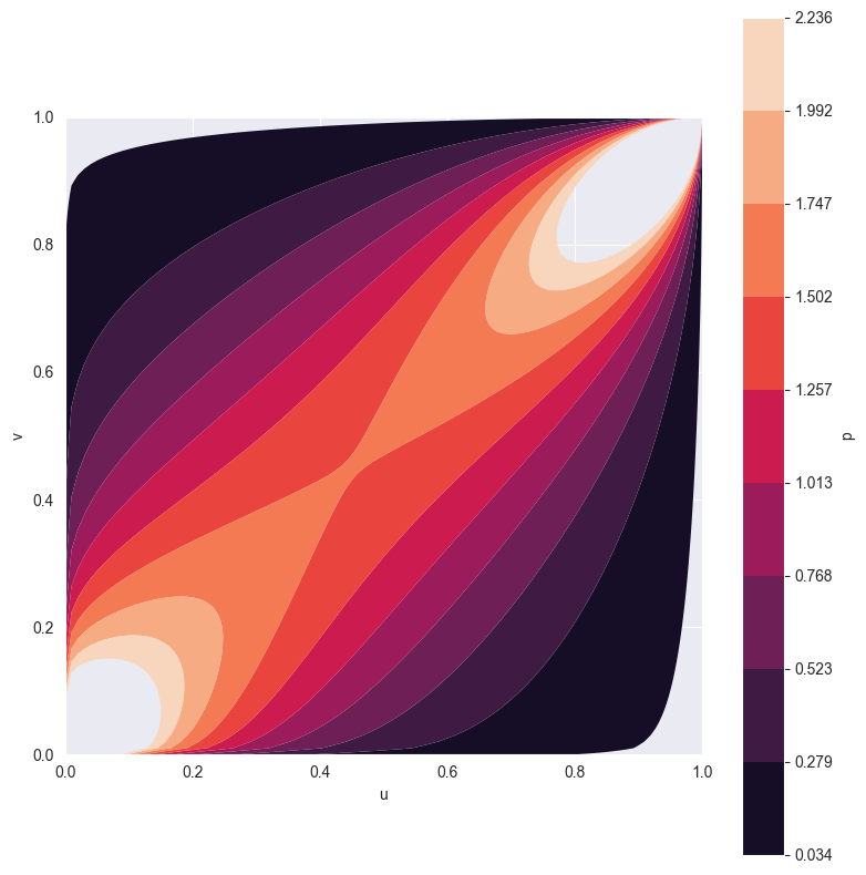
在这种情况下,我们使用Gumbel copula并固定其超参数theta=2。我们可以可视化其二维PDF。
[3]:
from statsmodels.distributions.copula.api import (
    CopulaDistribution, GumbelCopula, IndependenceCopula)

copula = GumbelCopula(theta=2)
_ = copula.plot_pdf()  # returns a matplotlib figure
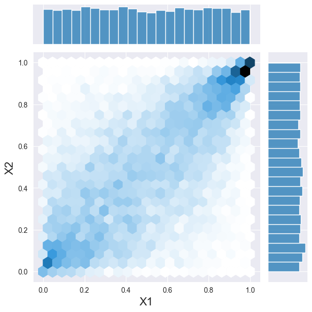
我们可以对PDF进行采样。
[4]:
sample = copula.rvs(10000)
h = sns.jointplot(x=sample[:, 0], y=sample[:, 1], kind="hex")
_ = h.set_axis_labels("X1", "X2", fontsize=16)
/Users/cw/baidu/code/fin_tool/github/statsmodels/venv/lib/python3.11/site-packages/statsmodels/tools/rng_qrng.py:54: FutureWarning: Passing `None` as the seed currently return the NumPy singleton RandomState
(np.random.mtrand._rand). After release 0.13 this will change to using the
default generator provided by NumPy (np.random.default_rng()). If you need
reproducible draws, you should pass a seeded np.random.Generator, e.g.,

import numpy as np
seed = 32839283923801
rng = np.random.default_rng(seed)"

  warnings.warn(_future_warn, FutureWarning)
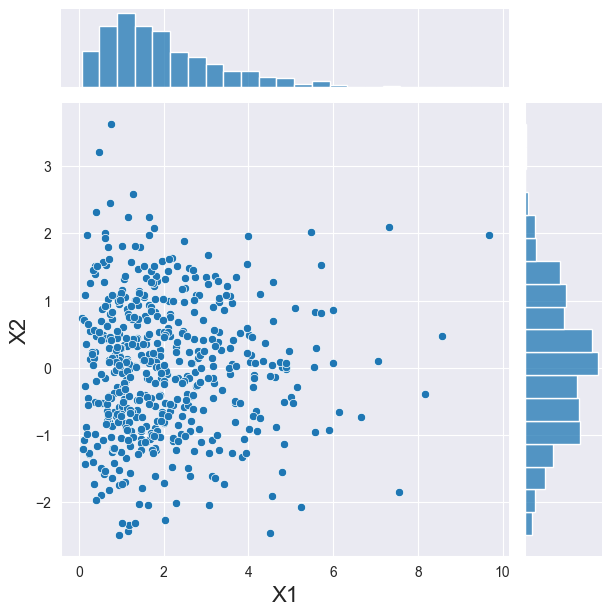
让我们回到我们的两个变量上来。在这种情况下,我们认为它们是伽马分布和正态分布的。如果它们彼此独立,我们可以分别从每个概率密度函数中进行采样。这里我们使用一个方便的类来执行相同的操作。
可重复性
从copulas生成可重复的随机值需要显式设置seed参数。seed接受一个已初始化的NumPy Generator或RandomState,或者任何可被np.random.default_rng接受的参数,例如一个整数或一个整数序列。此示例使用一个整数。
直接暴露在 np.random 分布中的单例 RandomState 未被使用,并且设置 np.random.seed 对生成的值没有影响。
[5]:
marginals = [stats.gamma(2), stats.norm]
joint_dist = CopulaDistribution(copula=IndependenceCopula(), marginals=marginals)
sample = joint_dist.rvs(512, random_state=20210801)
h = sns.jointplot(x=sample[:, 0], y=sample[:, 1], kind="scatter")
_ = h.set_axis_labels("X1", "X2", fontsize=16)
现在,我们在上面使用了一个copula来表示变量之间的依赖关系,我们可以使用这个copula来生成一组具有相同便利类别的新观测值。
[6]:
joint_dist = CopulaDistribution(copula, marginals)
# Use an initialized Generator object
rng = np.random.default_rng([2, 0, 2, 1, 0, 8, 0, 1])
sample = joint_dist.rvs(512, random_state=rng)
h = sns.jointplot(x=sample[:, 0], y=sample[:, 1], kind="scatter")
_ = h.set_axis_labels("X1", "X2", fontsize=16)
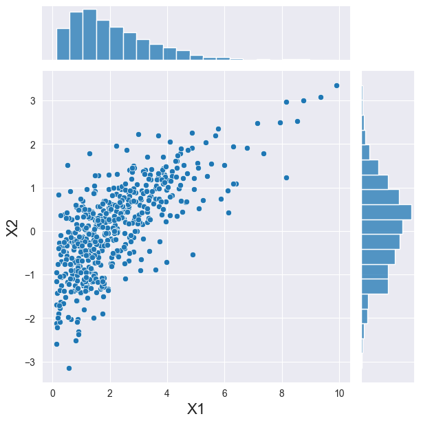
这里有两点需要注意。(i) 与独立情况一样,边缘分布正确显示了伽马分布和正态分布;(ii) 两个变量之间的依赖关系是可见的。
估计copula参数
现在,假设我们已经有了实验数据,并且我们知道存在一个可以用Gumbel copula表示的依赖关系。但我们不知道我们的copula的超参数值是多少。在这种情况下,我们可以估计这个值。
我们将使用刚刚生成的样本,因为我们已经知道我们应该得到的超参数值:theta=2。
[7]:
copula = GumbelCopula()
theta = copula.fit_corr_param(sample)
print(theta)
2.049379621506455
我们可以看到估计的超参数值接近之前设置的值。