ETS 模型
ETS 模型是一组基于状态空间模型的时间序列模型,该模型由一个水平分量、一个趋势分量(T)、一个季节性分量(S)和一个误差项(E)组成。
本笔记本展示了如何与statsmodels一起使用。对于更深入的处理,我们参考[1],第8章(免费在线资源),该章节是statsmodels中的实现以及本笔记本中使用的示例的基础。
statsmodels 实现了所有组合: - 加性和乘性误差模型 - 加性和乘性趋势,可能衰减 - 加性和乘性季节性
然而,并非所有这些方法都是稳定的。有关模型稳定性的更多信息,请参阅[1]及其参考文献。
[1] Hyndman, Rob J., 和 Athanasopoulos, George. 预测:原理与实践,第三版,OTexts, 2021. https://otexts.com/fpp3/expsmooth.html
[1]:
import numpy as np
import matplotlib.pyplot as plt
import pandas as pd

%matplotlib inline
from statsmodels.tsa.exponential_smoothing.ets import ETSModel
[2]:
plt.rcParams["figure.figsize"] = (12, 8)
简单指数平滑
最简单的ETS模型也被称为简单指数平滑。在ETS术语中,它对应于(A, N, N)模型,即具有加性误差、无趋势和无季节性的模型。Holt方法的状态空间公式如下:
\begin{align} y_{t} &= y_{t-1} + e_t\\ l_{t} &= l_{t-1} + \alpha e_t\\ \end{align}
这种状态空间公式可以转换为不同的公式,即预测和平滑方程(所有ETS模型都可以这样做):
\begin{align} \hat{y}_{t|t-1} &= l_{t-1}\\ l_{t} &= \alpha y_{t-1} + (1 - \alpha) l_{t-1} \end{align}
在这里,\(\hat{y}_{t|t-1}\) 是根据前一步信息对 \(y_t\) 的预测/期望。在简单指数平滑模型中,预测对应于前一个水平。第二个方程(平滑方程)计算下一个水平为前一个水平和前一个观测值的加权平均。
[3]:
oildata = [
    111.0091,
    130.8284,
    141.2871,
    154.2278,
    162.7409,
    192.1665,
    240.7997,
    304.2174,
    384.0046,
    429.6622,
    359.3169,
    437.2519,
    468.4008,
    424.4353,
    487.9794,
    509.8284,
    506.3473,
    340.1842,
    240.2589,
    219.0328,
    172.0747,
    252.5901,
    221.0711,
    276.5188,
    271.1480,
    342.6186,
    428.3558,
    442.3946,
    432.7851,
    437.2497,
    437.2092,
    445.3641,
    453.1950,
    454.4096,
    422.3789,
    456.0371,
    440.3866,
    425.1944,
    486.2052,
    500.4291,
    521.2759,
    508.9476,
    488.8889,
    509.8706,
    456.7229,
    473.8166,
    525.9509,
    549.8338,
    542.3405,
]
oil = pd.Series(oildata, index=pd.date_range("1965", "2013", freq="YS"))
oil.plot()
plt.ylabel("Annual oil production in Saudi Arabia (Mt)")
[3]:
Text(0, 0.5, 'Annual oil production in Saudi Arabia (Mt)')
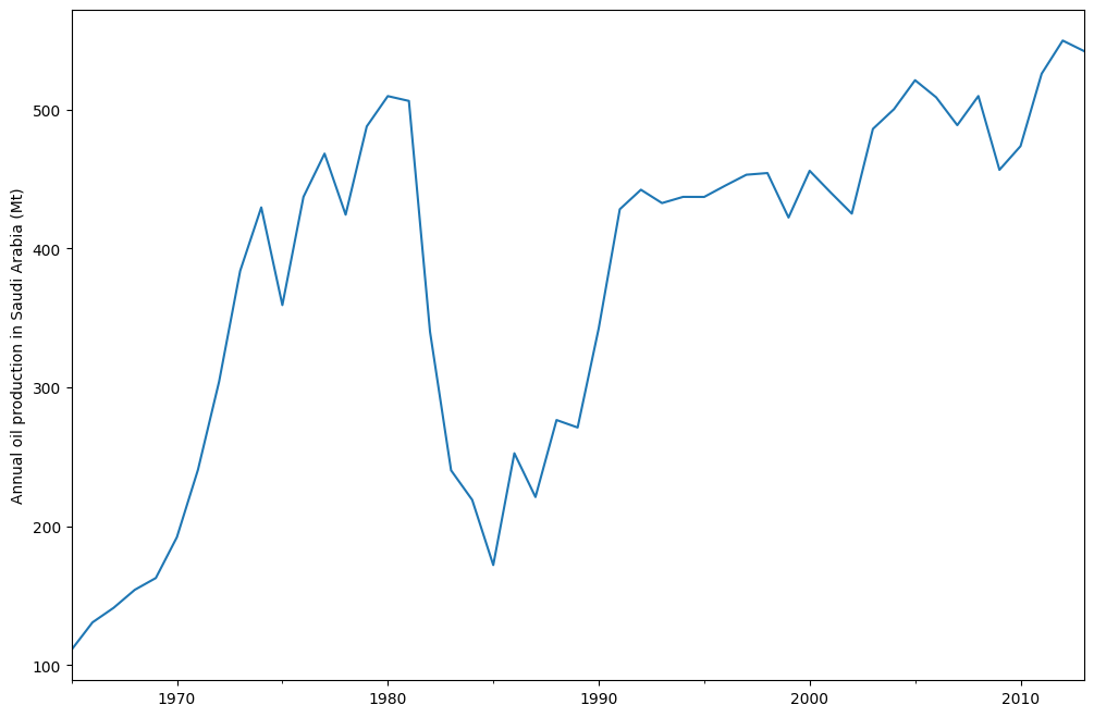
上图显示了沙特阿拉伯的年石油产量,单位为百万吨。数据来自R包fpp2(先前版本的配套包[1])。下面你可以看到如何使用statsmodels的ETS实现来拟合一个简单的指数平滑模型到这些数据。此外,还展示了使用R中的forecast进行拟合的比较。
[4]:
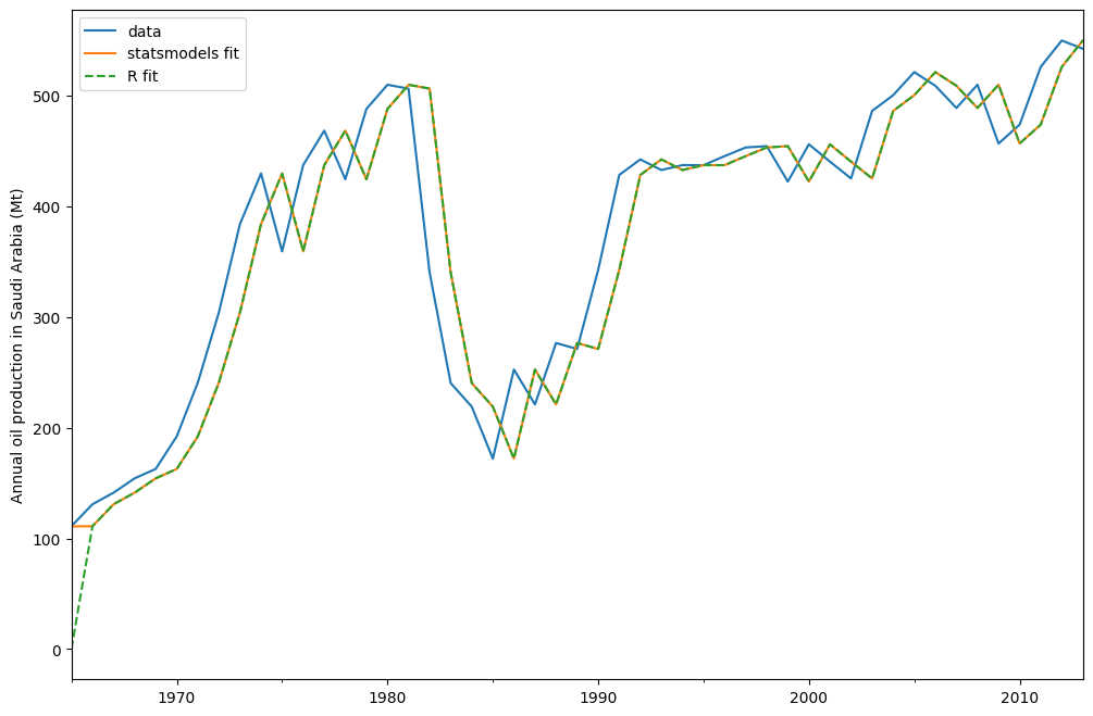
model = ETSModel(oil)
fit = model.fit(maxiter=10000)
oil.plot(label="data")
fit.fittedvalues.plot(label="statsmodels fit")
plt.ylabel("Annual oil production in Saudi Arabia (Mt)")

# obtained from R
params_R = [0.99989969, 0.11888177503085334, 0.80000197, 36.46466837, 34.72584983]
yhat = model.smooth(params_R).fittedvalues
yhat.plot(label="R fit", linestyle="--")

plt.legend()
RUNNING THE L-BFGS-B CODE

           * * *

Machine precision = 2.220D-16
 N =            2     M =           10

At X0         0 variables are exactly at the bounds

At iterate    0    f=  6.27365D+00    |proj g|=  8.99900D-01

At iterate    1    f=  5.31675D+00    |proj g|=  6.49880D-04

At iterate    2    f=  5.30939D+00    |proj g|=  5.55378D-04

At iterate    3    f=  5.29115D+00    |proj g|=  5.80869D-05

At iterate    4    f=  5.29096D+00    |proj g|=  2.04281D-06

           * * *

Tit   = total number of iterations
Tnf   = total number of function evaluations
Tnint = total number of segments explored during Cauchy searches
Skip  = number of BFGS updates skipped
Nact  = number of active bounds at final generalized Cauchy point
Projg = norm of the final projected gradient
F     = final function value

           * * *

   N    Tit     Tnf  Tnint  Skip  Nact     Projg        F
    2      4     13      5     0     1   2.043D-06   5.291D+00
  F =   5.2909564634118551

CONVERG
[4]:
<matplotlib.legend.Legend at 0x1044e3d10>
默认情况下,初始状态被视为拟合参数,并通过最大化对数似然来估计。也可以仅使用启发式方法来确定初始值:
[5]:
model_heuristic = ETSModel(oil, initialization_method="heuristic")
fit_heuristic = model_heuristic.fit()
oil.plot(label="data")
fit.fittedvalues.plot(label="estimated")
fit_heuristic.fittedvalues.plot(label="heuristic", linestyle="--")
plt.ylabel("Annual oil production in Saudi Arabia (Mt)")

# obtained from R
params = [0.99989969, 0.11888177503085334, 0.80000197, 36.46466837, 34.72584983]
yhat = model.smooth(params).fittedvalues
yhat.plot(label="with R params", linestyle=":")

plt.legend()
[5]:
<matplotlib.legend.Legend at 0x1166a3c90>
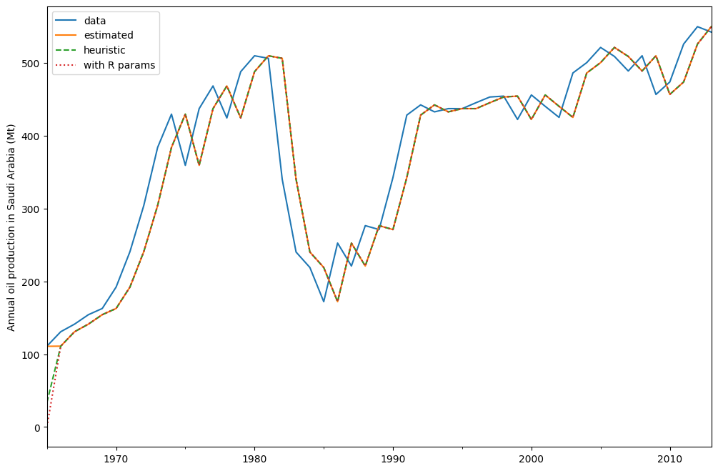
拟合参数和其他一些指标通过 fit.summary() 显示。在这里我们可以看到,使用拟合初始状态的模型的对数似然值略低于使用启发式初始状态的模型。
[6]:
print(fit.summary())
                                 ETS Results
==============================================================================
Dep. Variable:                      y   No. Observations:                   49
Model:                       ETS(ANN)   Log Likelihood                -259.257
Date:                Wed, 16 Oct 2024   AIC                            524.514
Time:                        18:27:49   BIC                            530.189
Sample:                    01-01-1965   HQIC                           526.667
                         - 01-01-2013   Scale                         2307.767
Covariance Type:               approx
===================================================================================
                      coef    std err          z      P>|z|      [0.025      0.975]
-----------------------------------------------------------------------------------
smoothing_level     0.9999      0.132      7.551      0.000       0.740       1.259
initial_level     110.7864     48.110      2.303      0.021      16.492     205.081
===================================================================================
Ljung-Box (Q):                        1.87   Jarque-Bera (JB):                20.78
Prob(Q):                              0.39   Prob(JB):                         0.00
Heteroskedasticity (H):               0.49   Skew:                            -1.04
Prob(H) (two-sided):                  0.16   Kurtosis:                         5.42
===================================================================================

Warnings:
[1] Covariance matrix calculated using numerical (complex-step) differentiation.
[7]:
print(fit_heuristic.summary())
                                 ETS Results
==============================================================================
Dep. Variable:                      y   No. Observations:                   49
Model:                       ETS(ANN)   Log Likelihood                -260.521
Date:                Wed, 16 Oct 2024   AIC                            525.042
Time:                        18:27:49   BIC                            528.826
Sample:                    01-01-1965   HQIC                           526.477
                         - 01-01-2013   Scale                         2429.964
Covariance Type:               approx
===================================================================================
                      coef    std err          z      P>|z|      [0.025      0.975]
-----------------------------------------------------------------------------------
smoothing_level     0.9999      0.132      7.559      0.000       0.741       1.259
==============================================
              initialization method: heuristic
----------------------------------------------
initial_level                          33.6309
===================================================================================
Ljung-Box (Q):                        1.85   Jarque-Bera (JB):                18.42
Prob(Q):                              0.40   Prob(JB):                         0.00
Heteroskedasticity (H):               0.44   Skew:                            -1.02
Prob(H) (two-sided):                  0.11   Kurtosis:                         5.21
===================================================================================

Warnings:
[1] Covariance matrix calculated using numerical (complex-step) differentiation.
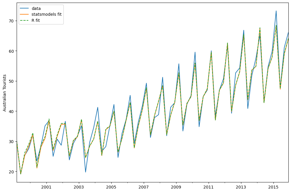
Holt-Winters’ 季节性方法
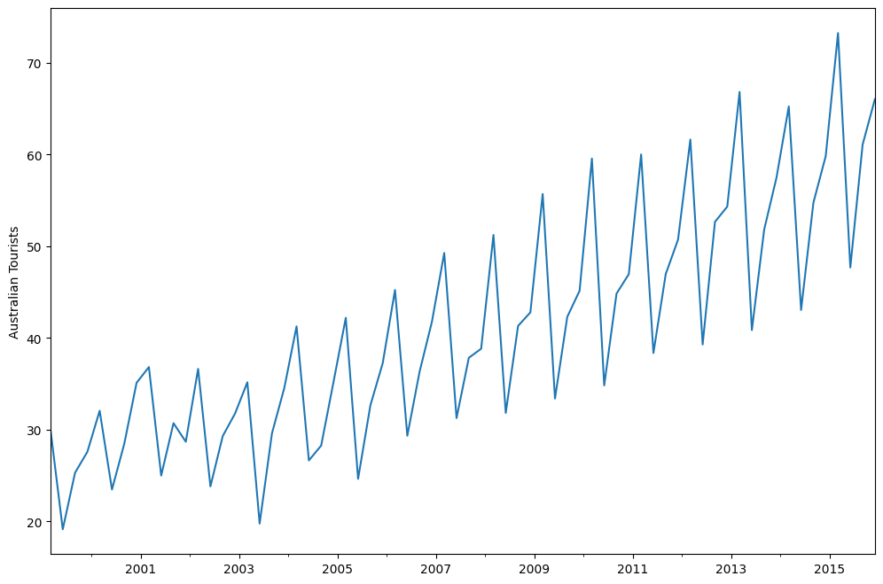
指数平滑法可以进行修改以包含趋势和季节性成分。在加性Holt-Winters方法中,季节性成分被添加到其余部分。该模型对应于ETS(A, A, A)模型,并具有以下状态空间公式:
\begin{align} y_t &= l_{t-1} + b_{t-1} + s_{t-m} + e_t\\ l_{t} &= l_{t-1} + b_{t-1} + \alpha e_t\\ b_{t} &= b_{t-1} + \beta e_t\\ s_{t} &= s_{t-m} + \gamma e_t \end{align}
[8]:
austourists_data = [
    30.05251300,
    19.14849600,
    25.31769200,
    27.59143700,
    32.07645600,
    23.48796100,
    28.47594000,
    35.12375300,
    36.83848500,
    25.00701700,
    30.72223000,
    28.69375900,
    36.64098600,
    23.82460900,
    29.31168300,
    31.77030900,
    35.17787700,
    19.77524400,
    29.60175000,
    34.53884200,
    41.27359900,
    26.65586200,
    28.27985900,
    35.19115300,
    42.20566386,
    24.64917133,
    32.66733514,
    37.25735401,
    45.24246027,
    29.35048127,
    36.34420728,
    41.78208136,
    49.27659843,
    31.27540139,
    37.85062549,
    38.83704413,
    51.23690034,
    31.83855162,
    41.32342126,
    42.79900337,
    55.70835836,
    33.40714492,
    42.31663797,
    45.15712257,
    59.57607996,
    34.83733016,
    44.84168072,
    46.97124960,
    60.01903094,
    38.37117851,
    46.97586413,
    50.73379646,
    61.64687319,
    39.29956937,
    52.67120908,
    54.33231689,
    66.83435838,
    40.87118847,
    51.82853579,
    57.49190993,
    65.25146985,
    43.06120822,
    54.76075713,
    59.83447494,
    73.25702747,
    47.69662373,
    61.09776802,
    66.05576122,
]
index = pd.date_range("1999-03-01", "2015-12-01", freq="3MS")
austourists = pd.Series(austourists_data, index=index)
austourists.plot()
plt.ylabel("Australian Tourists")
[8]:
Text(0, 0.5, 'Australian Tourists')
[9]:
# fit in statsmodels
model = ETSModel(
    austourists,
    error="add",
    trend="add",
    seasonal="add",
    damped_trend=True,
    seasonal_periods=4,
)
fit = model.fit()

# fit with R params
params_R = [
    0.35445427,
    0.03200749,
    0.39993387,
    0.97999997,
    24.01278357,
    0.97770147,
    1.76951063,
    -0.50735902,
    -6.61171798,
    5.34956637,
]
fit_R = model.smooth(params_R)

austourists.plot(label="data")
plt.ylabel("Australian Tourists")

fit.fittedvalues.plot(label="statsmodels fit")
fit_R.fittedvalues.plot(label="R fit", linestyle="--")
plt.legend()
[9]:
<matplotlib.legend.Legend at 0x11672bdd0>
[10]:
print(fit.summary())
                                 ETS Results
==============================================================================
Dep. Variable:                      y   No. Observations:                   68
Model:                      ETS(AAdA)   Log Likelihood                -152.627
Date:                Wed, 16 Oct 2024   AIC                            327.254
Time:                        18:27:50   BIC                            351.668
Sample:                    03-01-1999   HQIC                           336.928
                         - 12-01-2015   Scale                            5.213
Covariance Type:               approx
======================================================================================
                         coef    std err          z      P>|z|      [0.025      0.975]
--------------------------------------------------------------------------------------
smoothing_level        0.3399      0.111      3.070      0.002       0.123       0.557
smoothing_trend        0.0259      0.008      3.162      0.002       0.010       0.042
smoothing_seasonal     0.4010      0.080      5.041      0.000       0.245       0.557
damping_trend          0.9800        nan        nan        nan         nan         nan
initial_level         29.4450        nan        nan        nan         nan         nan
initial_trend          0.6143      0.392      1.566      0.117      -0.155       1.383
initial_seasonal.0    -3.4295        nan        nan        nan         nan         nan
initial_seasonal.1    -5.9545        nan        nan        nan         nan         nan
initial_seasonal.2   -11.4913        nan        nan        nan         nan         nan
initial_seasonal.3          0        nan        nan        nan         nan         nan
===================================================================================
Ljung-Box (Q):                        5.76   Jarque-Bera (JB):                 7.70
Prob(Q):                              0.67   Prob(JB):                         0.02
Heteroskedasticity (H):               0.46   Skew:                            -0.63
Prob(H) (two-sided):                  0.07   Kurtosis:                         4.05
===================================================================================

Warnings:
[1] Covariance matrix calculated using numerical (complex-step) differentiation.
预测
ETS模型也可以用于预测。有几种不同的方法可用:- forecast:进行样本外预测 - predict:样本内和样本外预测 - simulate:运行状态空间模型的模拟 - get_prediction:样本内和样本外预测,以及预测区间
我们可以在之前拟合的模型上使用它们来预测从2014年到2020年的数据。
[11]:
pred = fit.get_prediction(start="2014", end="2020")
[12]:
df = pred.summary_frame(alpha=0.05)
df
[12]:
| mean | pi_lower | pi_upper | |
|---|---|---|---|
| 2014-03-01 | 67.611216 | 63.136242 | 72.086191 |
| 2014-06-01 | 42.815135 | 38.340161 | 47.290109 |
| 2014-09-01 | 54.106583 | 49.631609 | 58.581558 |
| 2014-12-01 | 57.928184 | 53.453210 | 62.403158 |
| 2015-03-01 | 68.422418 | 63.947444 | 72.897392 |
| 2015-06-01 | 47.278586 | 42.803612 | 51.753561 |
| 2015-09-01 | 58.955314 | 54.480340 | 63.430289 |
| 2015-12-01 | 63.982579 | 59.507605 | 68.457553 |
| 2016-03-01 | 75.905700 | 71.430726 | 80.380674 |
| 2016-06-01 | 51.418965 | 46.654738 | 56.183192 |
| 2016-09-01 | 63.704186 | 58.630024 | 68.778348 |
| 2016-12-01 | 67.979000 | 62.576247 | 73.381754 |
| 2017-03-01 | 78.316987 | 71.736510 | 84.897463 |
| 2017-06-01 | 53.782026 | 46.884445 | 60.679607 |
| 2017-09-01 | 66.019986 | 58.789068 | 73.250904 |
| 2017-12-01 | 70.248484 | 62.669361 | 77.827607 |
| 2018-03-01 | 80.541081 | 71.893487 | 89.188675 |
| 2018-06-01 | 55.961638 | 46.969207 | 64.954069 |
| 2018-09-01 | 68.156006 | 58.805956 | 77.506055 |
| 2018-12-01 | 72.341783 | 62.622337 | 82.061229 |
| 2019-03-01 | 82.592514 | 71.865267 | 93.319761 |
| 2019-06-01 | 57.972043 | 46.876656 | 69.067429 |
| 2019-09-01 | 70.126202 | 58.652547 | 81.599858 |
| 2019-12-01 | 74.272576 | 62.411290 | 86.133862 |
| 2020-03-01 | 84.484691 | 71.656555 | 97.312827 |
在这种情况下,预测区间是使用一个解析公式计算的。并非所有模型都提供这种方法。对于这些其他模型,预测区间是通过执行多次模拟(默认情况下为1000次)并使用模拟结果的百分位数来计算的。这是由get_prediction方法在内部完成的。
我们也可以手动运行模拟,例如绘制它们。由于数据范围直到2015年底,我们必须从2016年第一季度模拟到2020年第一季度,这意味着17个步骤。
[13]:
simulated = fit.simulate(anchor="end", nsimulations=17, repetitions=100)
[14]:
for i in range(simulated.shape[1]):
    simulated.iloc[:, i].plot(label="_", color="gray", alpha=0.1)
df["mean"].plot(label="mean prediction")
df["pi_lower"].plot(linestyle="--", color="tab:blue", label="95% interval")
df["pi_upper"].plot(linestyle="--", color="tab:blue", label="_")
pred.endog.plot(label="data")
plt.legend()
[14]:
<matplotlib.legend.Legend at 0x116a73d10>
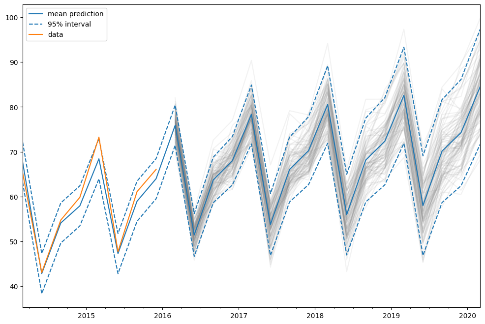
在这种情况下,我们选择“end”作为模拟锚点,这意味着第一个模拟值将是第一个样本外的值。也可以选择样本内的其他锚点。