GEE 得分检验
本笔记本使用模拟来演示稳健的GEE得分检验。这些检验可以在GEE分析中用于比较关于均值结构的嵌套假设。这些检验对于工作相关性模型的错误指定具有稳健性,并且对于方差结构的某些形式的错误指定也具有稳健性(例如,在准泊松分析中通过尺度参数捕获的错误指定)。
数据被模拟为集群,其中集群内部存在依赖性,但集群之间不存在依赖性。集群内的依赖性是通过copula方法引入的。数据边缘上遵循负二项分布(gamma/Poisson混合)。
以下考虑了测试的水平和能力,以评估测试的性能。
[1]:
import pandas as pd
import numpy as np
from scipy.stats.distributions import norm, poisson
import statsmodels.api as sm
import matplotlib.pyplot as plt
以下单元格中定义的函数使用copula方法来模拟边缘服从负二项分布的相关随机值。输入参数u是一个(0, 1)范围内的值数组。u的元素必须在(0, 1)上边缘均匀分布。u中的相关性将导致返回的负二项值的相关性。数组参数mu给出边缘均值,标量参数scale定义均值/方差关系(方差是均值的scale倍)。u和mu的长度必须相同。
[2]:
def negbinom(u, mu, scale):
    p = (scale - 1) / scale
    r = mu * (1 - p) / p
    x = np.random.gamma(r, p / (1 - p), len(u))
    return poisson.ppf(u, mu=x)
以下是一些控制模拟中使用的数据的参数。
[3]:
# Sample size
n = 1000

# Number of covariates (including intercept) in the alternative hypothesis model
p = 5

# Cluster size
m = 10

# Intraclass correlation (controls strength of clustering)
r = 0.5

# Group indicators
grp = np.kron(np.arange(n/m), np.ones(m))
该模拟使用一个固定设计矩阵。
[4]:
# Build a design matrix for the alternative (more complex) model
x = np.random.normal(size=(n, p))
x[:, 0] = 1
零假设设计矩阵嵌套在备择假设设计矩阵中。它的秩比备择假设设计矩阵少两个。
[5]:
x0 = x[:, 0:3]
GEE 得分检验对依赖性和过度分散具有鲁棒性。这里我们设置过度分散参数。每个观测值的负二项分布的方差等于 scale 乘以其均值。
[6]:
# Scale parameter for negative binomial distribution
scale = 10
在下一个单元格中,我们为零假设模型和备择模型设置了均值结构
[7]:
# The coefficients used to define the linear predictors
coeff = [[4, 0.4, -0.2], [4, 0.4, -0.2, 0, -0.04]]

# The linear predictors
lp = [np.dot(x0, coeff[0]), np.dot(x, coeff[1])]

# The mean values
mu = [np.exp(lp[0]), np.exp(lp[1])]
下面是一个执行模拟的函数。
[8]:
# hyp = 0 is the null hypothesis, hyp = 1 is the alternative hypothesis.
# cov_struct is a statsmodels covariance structure
def dosim(hyp, cov_struct=None, mcrep=500):

    # Storage for the simulation results
    scales = [[], []]

    # P-values from the score test
    pv = []

    # Monte Carlo loop
    for k in range(mcrep):

        # Generate random "probability points" u  that are uniformly
        # distributed, and correlated within clusters
        z = np.random.normal(size=n)
        u = np.random.normal(size=n//m)
        u = np.kron(u, np.ones(m))
        z = r*z +np.sqrt(1-r**2)*u
        u = norm.cdf(z)

        # Generate the observed responses
        y = negbinom(u, mu=mu[hyp], scale=scale)

        # Fit the null model
        m0 = sm.GEE(y, x0, groups=grp, cov_struct=cov_struct, family=sm.families.Poisson())
        r0 = m0.fit(scale='X2')
        scales[0].append(r0.scale)

        # Fit the alternative model
        m1 = sm.GEE(y, x, groups=grp, cov_struct=cov_struct, family=sm.families.Poisson())
        r1 = m1.fit(scale='X2')
        scales[1].append(r1.scale)

        # Carry out the score test
        st = m1.compare_score_test(r0)
        pv.append(st["p-value"])

    pv = np.asarray(pv)
    rslt = [np.mean(pv), np.mean(pv < 0.1)]

    return rslt, scales
使用独立工作协方差结构运行模拟。在零假设下,我们预期均值大约为0,而在备择假设下,均值会低得多。同样,我们预期在零假设下,大约10%的p值小于0.1,而在备择假设下,p值小于0.1的比例会大得多。
[9]:
rslt, scales = [], []

for hyp in 0, 1:
    s, t = dosim(hyp, sm.cov_struct.Independence())
    rslt.append(s)
    scales.append(t)

rslt = pd.DataFrame(rslt, index=["H0", "H1"], columns=["Mean", "Prop(p<0.1)"])

print(rslt)
        Mean  Prop(p<0.1)
H0  0.495237        0.100
H1  0.037242        0.896
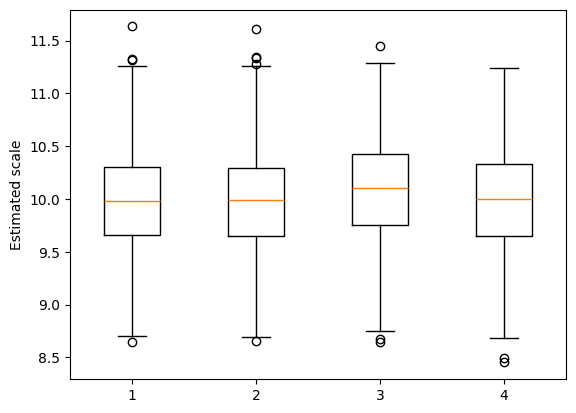
接下来我们检查以确保尺度参数估计是合理的。我们正在评估GEE得分检验对依赖性和过度离散的稳健性,因此这里我们确认过度离散如预期存在。
[10]:
_ = plt.boxplot([scales[0][0], scales[0][1], scales[1][0], scales[1][1]])
plt.ylabel("Estimated scale")
[10]:
Text(0, 0.5, 'Estimated scale')
接下来,我们使用可交换的工作相关性模型进行相同的分析。请注意,这将比使用独立工作相关性的上述示例慢,因此我们使用较少的蒙特卡洛重复次数。
[11]:
rslt, scales = [], []

for hyp in 0, 1:
    s, t = dosim(hyp, sm.cov_struct.Exchangeable(), mcrep=100)
    rslt.append(s)
    scales.append(t)

rslt = pd.DataFrame(rslt, index=["H0", "H1"], columns=["Mean", "Prop(p<0.1)"])

print(rslt)
        Mean  Prop(p<0.1)
H0  0.526654         0.11
H1  0.042463         0.88