事后估计概述 - 泊松
本笔记本提供了几个模型中可用的后估计结果的概述,以泊松模型为例进行了说明。
参见 https://github.com/statsmodels/statsmodels/issues/7707
传统上,模型提供的 Wald 推断和预测的结果类。现在,几个模型有用于推断、预测和规范或诊断测试的后估计结果的附加方法。
以下内容基于tsa之外的最大似然模型的当前模式,主要针对离散模型。其他模型在某种程度上仍然遵循不同的API模式。例如,OLS和WLS等线性模型有其特殊的实现,如OLS影响。GLM也仍然有一些特定于模型的功能。
主要的估计后功能包括
推断 - Wald 检验 部分
推断 - 得分检验 部分
get_prediction带有推断统计的预测 部分get_distribution基于估计参数的分布类 部分get_diagnostic诊断和规范测试、度量和图表 部分get_influence异常值和影响诊断 部分
一个模拟的例子
为了说明,我们模拟了泊松回归的数据,该回归正确指定并且具有相对较大的样本。一个回归变量是具有两个水平的分类变量,第二个回归变量在单位区间上均匀分布。
[1]:
import numpy as np
import pandas as pd
from scipy import stats
import matplotlib.pyplot as plt

from statsmodels.discrete.discrete_model import Poisson
from statsmodels.discrete.diagnostic import PoissonDiagnostic
[2]:
np.random.seed(983154356)

nr = 10
n_groups = 2
labels = np.arange(n_groups)
x = np.repeat(labels, np.array([40, 60]) * nr)
nobs = x.shape[0]
exog = (x[:, None] == labels).astype(np.float64)
xc = np.random.rand(len(x))
exog = np.column_stack((exog, xc))
# reparameterize to explicit constant
# exog[:, 1] = 1
beta = np.array([0.2, 0.3, 0.5], np.float64)

linpred = exog @ beta
mean = np.exp(linpred)
y = np.random.poisson(mean)
len(y), y.mean(), (y == 0).mean()

res = Poisson(y, exog).fit(disp=0)
print(res.summary())
                          Poisson Regression Results
==============================================================================
Dep. Variable:                      y   No. Observations:                 1000
Model:                        Poisson   Df Residuals:                      997
Method:                           MLE   Df Model:                            2
Date:                Wed, 16 Oct 2024   Pseudo R-squ.:                 0.01258
Time:                        18:27:38   Log-Likelihood:                -1618.3
converged:                       True   LL-Null:                       -1638.9
Covariance Type:            nonrobust   LLR p-value:                 1.120e-09
==============================================================================
                 coef    std err          z      P>|z|      [0.025      0.975]
------------------------------------------------------------------------------
x1             0.2386      0.061      3.926      0.000       0.120       0.358
x2             0.3229      0.055      5.873      0.000       0.215       0.431
x3             0.5109      0.083      6.186      0.000       0.349       0.673
==============================================================================
[ ]:
推理 - 沃尔德
cov_type option for fit).目前可用的方法,除了参数表中的统计数据外,还有
t检验
wald_test
成对t检验
wald_test_terms
f_test 是一个可用的传统方法。它与 wald_test 相同,使用关键字选项 use_f=True。
[3]:
res.t_test("x1=x2")
[3]:
<class 'statsmodels.stats.contrast.ContrastResults'>
                             Test for Constraints
==============================================================================
                 coef    std err          z      P>|z|      [0.025      0.975]
------------------------------------------------------------------------------
c0            -0.0843      0.049     -1.717      0.086      -0.181       0.012
==============================================================================
[4]:
res.wald_test("x1=x2, x3", scalar=True)
[4]:
<class 'statsmodels.stats.contrast.ContrastResults'>
<Wald test (chi2): statistic=40.772322944293144, p-value=1.4008852592192469e-09, df_denom=2>
推理 - score_test
statsmodels 0.14 中新增的功能,适用于大多数离散模型和 GLM。
得分或拉格朗日乘数(LM)检验基于在零假设下估计的模型。一个常见的例子是变量添加检验,在这种检验中,我们在零假设的限制下估计模型参数,但在全模型下评估得分和海森矩阵,以检验是否添加的变量在统计上是显著的。
cov_type for Wald tests will not be appropriate for score tests. In many cases Wald tests overjects but score tests can underreject. Using the Wald small sample corrections for score tests might leads then to more conservative p-values.我们可以使用变量 addition score_test 进行规范测试。在下面的示例中,我们通过添加二次或多项式项来测试模型中是否存在某些未正确指定的非线性。
在我们的示例中,我们可以预期这些规范测试不会拒绝原假设,因为模型是正确指定的,并且样本量很大,
[5]:
res.score_test(exog_extra=xc**2)
[5]:
(array([0.05300569]), array([0.81791332]), 1)
[6]:
linpred = res.predict(which="linear")
res.score_test(exog_extra=linpred[:,None]**[2, 3])
[6]:
(array([1.3867703]), array([0.49988103]), 2)
预测
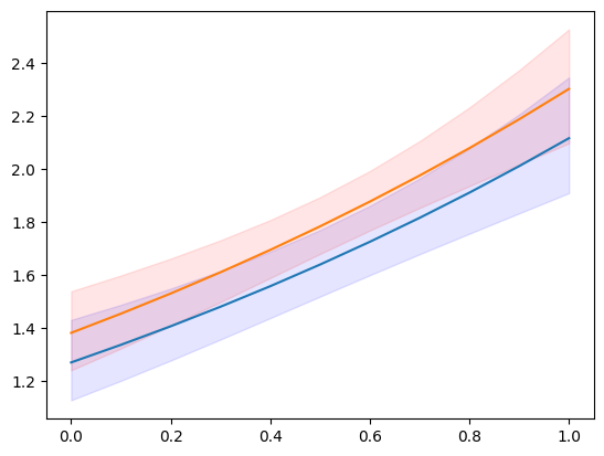
模型和结果类具有 predict 方法,该方法仅返回预测值。get_prediction 方法为预测添加了推断统计量、标准误差、p值和置信区间。
对于以下示例,我们创建了新的解释变量集,这些变量集按分类级别划分,并在连续变量的均匀网格上进行划分。
[7]:
n = 11
exc = np.linspace(0, 1, n)
ex1 = np.column_stack((np.ones(n), np.zeros(n), exc))
ex2 = np.column_stack((np.zeros(n), np.ones(n), exc))

m1 = res.get_prediction(ex1)
m2 = res.get_prediction(ex2)
预测结果类的可用方法和属性有
[8]:
[i for i in dir(m1) if not i.startswith("_")]
[8]:
['conf_int',
 'deriv',
 'df',
 'dist',
 'dist_args',
 'func',
 'linpred',
 'linpred_se',
 'predicted',
 'row_labels',
 'se',
 'summary_frame',
 't_test',
 'tvalues',
 'var_pred']
[9]:
plt.plot(exc, np.column_stack([m1.predicted, m2.predicted]))
ci = m1.conf_int()
plt.fill_between(exc, ci[:, 0], ci[:, 1], color='b', alpha=.1)
ci = m2.conf_int()
plt.fill_between(exc, ci[:, 0], ci[:, 1], color='r', alpha=.1)
# to add observed points:
# y1 = y[x == 0]
# plt.plot(xc[x == 0], y1, ".", color="b", alpha=.3)
# y2 = y[x == 1]
# plt.plot(xc[x == 1], y2, ".", color="r", alpha=.3)
[9]:
<matplotlib.collections.PolyCollection at 0x11fc5a790>
[10]:
y.max()
[10]:
np.int64(7)
我们可以预测的可用统计数据之一,由“which”关键字指定,是预测分布的期望频率或概率。这向我们展示了在给定一组解释变量的情况下,观察计数为1、2、3等的预测概率。
[11]:
y_max = 5
f1 = res.get_prediction(ex1, which="prob", y_values=np.arange(y_max + 1))
f2 = res.get_prediction(ex2, which="prob", y_values=np.arange(y_max + 1))
f1.predicted.mean(0), f2.predicted.mean(0)
[11]:
(array([0.19681697, 0.31325239, 0.25570764, 0.14275759, 0.06128168,
        0.02154715]),
 array([0.17115113, 0.29529781, 0.26128059, 0.15810937, 0.07357482,
        0.02804883]))
我们也可以获得预测概率的置信区间。然而,如果我们想要平均预测概率的置信区间,那么我们需要在预测函数内部进行聚合。相关的关键词是“average”,它计算在由exog数组给出的观测值上的预测的平均值。
[12]:
f1 = res.get_prediction(ex1, which="prob", y_values=np.arange(y_max + 1), average=True)
f2 = res.get_prediction(ex2, which="prob", y_values=np.arange(y_max + 1), average=True)
f1.predicted, f2.predicted
[12]:
(array([0.19681697, 0.31325239, 0.25570764, 0.14275759, 0.06128168,
        0.02154715]),
 array([0.17115113, 0.29529781, 0.26128059, 0.15810937, 0.07357482,
        0.02804883]))
[13]:
f1.conf_int()
[13]:
array([[0.17256941, 0.22106453],
       [0.2982307 , 0.32827408],
       [0.24818616, 0.26322912],
       [0.12876732, 0.15674787],
       [0.05088296, 0.07168041],
       [0.01626921, 0.0268251 ]])
[14]:
f2.conf_int()
[14]:
array([[0.15303084, 0.18927142],
       [0.28178041, 0.30881522],
       [0.25622062, 0.26634055],
       [0.14720224, 0.1690165 ],
       [0.06442055, 0.0827291 ],
       [0.02287077, 0.03322688]])
help(res.get_prediction)help(res.model.predict)分布
对于给定的参数,我们可以创建一个scipy或scipy兼容的分布类实例。这使我们能够访问分布中的任何方法,如pmf/pdf、cdf、stats。
结果类的 get_distribution 方法使用提供的解释变量数组和估计的参数来指定一个矢量化的分布。模型的 get_prediction 方法可以用于用户指定的参数 params。
[15]:
distr = res.get_distribution()
distr
[15]:
<scipy.stats._distn_infrastructure.rv_discrete_frozen at 0x11e47d4d0>
[16]:
distr.pmf(0)[:10]
[16]:
array([0.15420516, 0.13109359, 0.17645042, 0.16735421, 0.13445031,
       0.14851843, 0.22287053, 0.14979318, 0.25252986, 0.25013583])
条件分布的均值与模型预测的均值相同。
[17]:
distr.mean()[:10]
[17]:
array([1.86947133, 2.03184379, 1.73471534, 1.78764267, 2.00656061,
       1.90704623, 1.50116427, 1.89849971, 1.37622577, 1.3857512 ])
[18]:
res.predict()[:10]
[18]:
array([1.86947133, 2.03184379, 1.73471534, 1.78764267, 2.00656061,
       1.90704623, 1.50116427, 1.89849971, 1.37622577, 1.3857512 ])
我们也可以为一组新的解释变量获得分布。解释变量可以以与预测方法相同的方式提供。
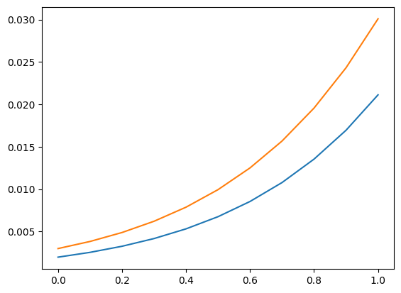
我们再次使用预测部分中的解释变量网格。作为一个使用示例,我们可以计算在解释变量的值条件下,观察到严格大于5的计数的概率。
[19]:
distr1 = res.get_distribution(ex1)
distr2 = res.get_distribution(ex2)
[20]:
distr1.sf(5), distr2.sf(5)
[20]:
(array([0.00198421, 0.00255027, 0.00326858, 0.00417683, 0.00532093,
        0.00675641, 0.00854998, 0.01078116, 0.0135439 , 0.01694825,
        0.02112179]),
 array([0.00299758, 0.00383456, 0.00489029, 0.00621677, 0.00787663,
        0.00994468, 0.01250966, 0.01567579, 0.01956437, 0.02431503,
        0.03008666]))
[21]:
plt.plot(exc, np.column_stack([distr1.sf(5), distr2.sf(5)]))
[21]:
[<matplotlib.lines.Line2D at 0x11fd19010>,
 <matplotlib.lines.Line2D at 0x11fd19390>]
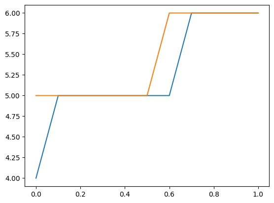
我们也可以使用分布来找到一个新的观测值的上限置信区间。以下图表显示了给定解释变量的上限计数。观测到此计数或更少的概率至少为0.99。
注意,这假设参数是固定的,并不考虑参数的不确定性。
[22]:
plt.plot(exc, np.column_stack([distr1.ppf(0.99), distr2.ppf(0.99)]))
[22]:
[<matplotlib.lines.Line2D at 0x11fd7d8d0>,
 <matplotlib.lines.Line2D at 0x11fd2f410>]
[23]:
[distr1.ppf(0.99), distr2.ppf(0.99)]
[23]:
[array([4., 5., 5., 5., 5., 5., 5., 6., 6., 6., 6.]),
 array([5., 5., 5., 5., 5., 5., 6., 6., 6., 6., 6.])]
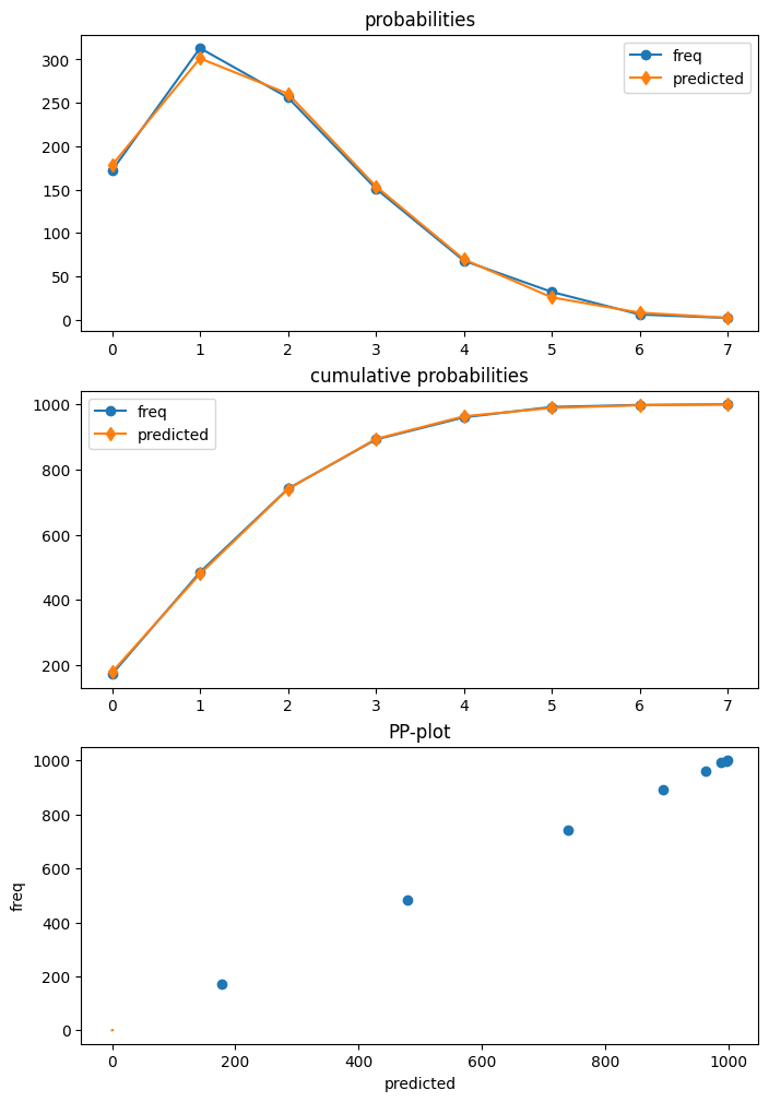
诊断
泊松是第一个具有诊断类别的模型,可以通过使用get_diagnostic从结果中获得。其他计数模型有一个通用的计数诊断类别,目前只有有限数量的方法。
在我们的示例中,泊松模型被正确指定。此外,我们有一个较大的样本量。因此,在这种情况下,没有任何诊断测试拒绝正确指定的原假设。
[24]:
dia = res.get_diagnostic()
[i for i in dir(dia) if not i.startswith("_")]
[24]:
['plot_probs',
 'probs_predicted',
 'results',
 'test_chisquare_prob',
 'test_dispersion',
 'test_poisson_zeroinflation',
 'y_max']
[25]:
dia.plot_probs();
过度分散测试
有几种用于泊松分布的离散度检验方法。目前所有这些方法都会返回结果。DispersionResults 类有一个 summary_frame 方法。返回的数据框提供了更易读的结果概览。
[26]:
td = dia.test_dispersion()
td
[26]:
<class 'statsmodels.discrete._diagnostics_count.DispersionResults'>
statistic = array([-0.42597379, -0.42597379, -0.39884024, -0.48327447, -0.48327447,
           -0.47790855, -0.45225818])
pvalue = array([0.67012695, 0.67012695, 0.69001092, 0.62890087, 0.62890087,
           0.6327153 , 0.651083  ])
method = ['Dean A', 'Dean B', 'Dean C', 'CT nb2', 'CT nb1', 'CT nb2 HC3', 'CT nb1 HC3']
alternative = ['mu (1 + a mu)', 'mu (1 + a mu)', 'mu (1 + a)', 'mu (1 + a mu)', 'mu (1 + a)', 'mu (1 + a mu)', 'mu (1 + a)']
name = 'Poisson Dispersion Test'
tuple = (array([-0.42597379, -0.42597379, -0.39884024, -0.48327447, -0.48327447,
           -0.47790855, -0.45225818]), array([0.67012695, 0.67012695, 0.69001092, 0.62890087, 0.62890087,
           0.6327153 , 0.651083  ]))
[27]:
df = td.summary_frame()
df
[27]:
| statistic | pvalue | method | alternative | |
|---|---|---|---|---|
| 0 | -0.425974 | 0.670127 | Dean A | mu (1 + a mu) |
| 1 | -0.425974 | 0.670127 | Dean B | mu (1 + a mu) |
| 2 | -0.398840 | 0.690011 | Dean C | mu (1 + a) |
| 3 | -0.483274 | 0.628901 | CT nb2 | mu (1 + a mu) |
| 4 | -0.483274 | 0.628901 | CT nb1 | mu (1 + a) |
| 5 | -0.477909 | 0.632715 | CT nb2 HC3 | mu (1 + a mu) |
| 6 | -0.452258 | 0.651083 | CT nb1 HC3 | mu (1 + a) |
零膨胀测试
[28]:
dia.test_poisson_zeroinflation()
[28]:
<class 'statsmodels.stats.base.HolderTuple'>
statistic = np.float64(-0.6657556201098715)
pvalue = np.float64(0.5055673158225649)
pvalue_smaller = np.float64(0.7472163420887176)
pvalue_larger = np.float64(0.25278365791128243)
chi2 = np.float64(0.4432305457078796)
pvalue_chi2 = np.float64(0.5055673158225649)
df_chi2 = 1
distribution = 'normal'
tuple = (np.float64(-0.6657556201098715), np.float64(0.5055673158225649))
零膨胀的卡方检验
[29]:
dia.test_chisquare_prob(bin_edges=np.arange(3))
[29]:
<class 'statsmodels.stats.base.HolderTuple'>
statistic = np.float64(0.45617094187322405)
pvalue = np.float64(0.49941894681204924)
df = np.int64(1)
diff1 = array([[-0.15420516,  0.71171787],
           [-0.13109359, -0.26636169],
           [-0.17645042, -0.30609125],
           ...,
           [-0.10477112, -0.23636125],
           [-0.10675436, -0.2388335 ],
           [-0.21168332, -0.32867305]])
res_aux = <statsmodels.regression.linear_model.RegressionResultsWrapper object at 0x11ff04390>
distribution = 'chi2'
tuple = (np.float64(0.45617094187322405), np.float64(0.49941894681204924))
预测频率的拟合优度检验
这是一个考虑参数估计的卡方检验。大于最大箱边缘的计数将被添加到最后一个箱中,以使箱的总和为一。
例如使用5个区间
[30]:
dt = dia.test_chisquare_prob(bin_edges=np.arange(6))
dt
[30]:
<class 'statsmodels.stats.base.HolderTuple'>
statistic = np.float64(0.9414641297778026)
pvalue = np.float64(0.918538200834608)
df = np.int64(4)
diff1 = array([[-0.15420516,  0.71171787, -0.26946759, -0.16792064, -0.07848071],
           [-0.13109359, -0.26636169, -0.27060268,  0.81672588, -0.0930961 ],
           [-0.17645042, -0.30609125,  0.7345094 , -0.15351687, -0.06657702],
           ...,
           [-0.10477112, -0.23636125, -0.26661279,  0.79950922, -0.11307565],
           [-0.10675436, -0.2388335 ,  0.73283789, -0.1992339 , -0.11143275],
           [-0.21168332, -0.32867305,  0.74484061, -0.13205892, -0.05126078]])
res_aux = <statsmodels.regression.linear_model.RegressionResultsWrapper object at 0x11ff04910>
distribution = 'chi2'
tuple = (np.float64(0.9414641297778026), np.float64(0.918538200834608))
[31]:
dt.diff1.mean(0)
[31]:
array([-0.00628136, 0.01177308, -0.00449604, -0.00270524, -0.00156519])
[32]:
vars(dia)
[32]:
{'results': <statsmodels.discrete.discrete_model.PoissonResults at 0x11df253d0>,
 'y_max': None,
 '_cache': {'probs_predicted': array([[0.15420516, 0.28828213, 0.26946759, ..., 0.02934349, 0.0091428 ,
          0.00244174],
         [0.13109359, 0.26636169, 0.27060268, ..., 0.03783135, 0.01281123,
          0.00371863],
         [0.17645042, 0.30609125, 0.2654906 , ..., 0.02309843, 0.0066782 ,
          0.00165497],
         ...,
         [0.10477112, 0.23636125, 0.26661279, ..., 0.05101921, 0.01918303,
          0.00618235],
         [0.10675436, 0.2388335 , 0.26716211, ..., 0.04986002, 0.01859135,
          0.00594186],
         [0.21168332, 0.32867305, 0.25515939, ..., 0.01591815, 0.00411926,
          0.00091369]])}}
异常值和影响
Statsmodels 提供了一个通用的 MLEInfluence 类,用于非线性模型(具有非线性期望均值的模型),适用于离散模型和其他基于最大似然估计的模型,例如 Beta 回归模型。提供的度量基于一般定义,例如广义杠杆,而不是线性模型中帽子矩阵的对角线。
结果方法 get_influence 返回一个 MLEInfluence 类的实例,该类具有用于异常值和影响度量的各种方法。
[33]:
infl = res.get_influence()
[i for i in dir(infl) if not i.startswith("_")]
[33]:
['cooks_distance',
 'cov_params',
 'd_fittedvalues',
 'd_fittedvalues_scaled',
 'd_params',
 'dfbetas',
 'endog',
 'exog',
 'hat_matrix_diag',
 'hat_matrix_exog_diag',
 'hessian',
 'k_params',
 'k_vars',
 'model_class',
 'nobs',
 'params_one',
 'plot_index',
 'plot_influence',
 'resid',
 'resid_score',
 'resid_score_factor',
 'resid_studentized',
 'results',
 'scale',
 'score_obs',
 'summary_frame']
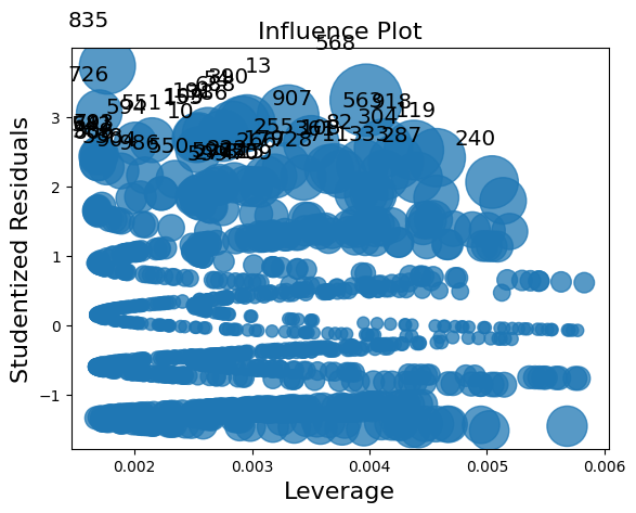
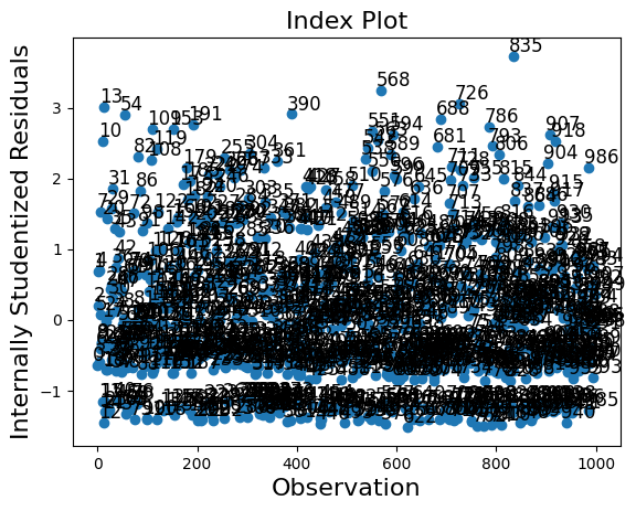
influence 类有两个绘图方法。然而,由于样本量较大,在这种情况下图表显得过于拥挤。
[34]:
infl.plot_influence();
[35]:
infl.plot_index(y_var="resid_studentized");
一个 summary_frame 显示了每个观测值的主要影响和异常值度量。
在我们的示例中,我们有1000个观测值,这太多了,无法轻松显示。我们可以按某一列对汇总数据框进行排序,并列出具有最大异常值或影响度量的观测值。在下面的示例中,我们按Cook’s距离和standard_resid排序,后者在一般情况下是Pearson残差。
因为我们模拟了一个“良好”的模型,所以没有具有较大影响或为较大异常值的观测结果。
[36]:
df_infl = infl.summary_frame()
df_infl.head()
[36]:
| dfb_x1 | dfb_x2 | dfb_x3 | cooks_d | standard_resid | hat_diag | dffits_internal | |
|---|---|---|---|---|---|---|---|
| 0 | -0.010856 | 0.011384 | -0.013643 | 0.000440 | -0.636944 | 0.003243 | -0.036334 |
| 1 | 0.001990 | -0.023625 | 0.028313 | 0.000737 | 0.680823 | 0.004749 | 0.047031 |
| 2 | 0.005794 | -0.000787 | 0.000943 | 0.000035 | 0.201681 | 0.002607 | 0.010311 |
| 3 | -0.014243 | 0.005539 | -0.006639 | 0.000325 | -0.589923 | 0.002790 | -0.031206 |
| 4 | 0.003602 | -0.022549 | 0.027024 | 0.000738 | 0.702888 | 0.004462 | 0.047057 |
[37]:
df_infl.sort_values("cooks_d", ascending=False)[:10]
[37]:
| dfb_x1 | dfb_x2 | dfb_x3 | cooks_d | standard_resid | hat_diag | dffits_internal | |
|---|---|---|---|---|---|---|---|
| 568 | -0.110520 | -0.038997 | 0.143106 | 0.013922 | 3.236167 | 0.003972 | 0.204365 |
| 13 | 0.048914 | -0.056713 | 0.067969 | 0.010034 | 3.011778 | 0.003307 | 0.173497 |
| 918 | -0.093971 | -0.038431 | 0.121677 | 0.009304 | 2.519367 | 0.004378 | 0.167066 |
| 563 | -0.089917 | -0.033708 | 0.116428 | 0.008935 | 2.545624 | 0.004119 | 0.163720 |
| 119 | 0.163230 | 0.103957 | -0.124589 | 0.008883 | 2.409646 | 0.004569 | 0.163247 |
| 390 | 0.148697 | 0.066972 | -0.080264 | 0.008358 | 2.907190 | 0.002958 | 0.158345 |
| 835 | -0.017672 | 0.066475 | 0.022883 | 0.008209 | 3.727645 | 0.001769 | 0.156931 |
| 54 | 0.145944 | 0.064216 | -0.076961 | 0.008156 | 2.892554 | 0.002916 | 0.156419 |
| 907 | -0.078901 | -0.020908 | 0.102164 | 0.008021 | 2.615676 | 0.003505 | 0.155126 |
| 304 | 0.152905 | 0.093680 | -0.112272 | 0.007821 | 2.351520 | 0.004225 | 0.153179 |
[38]:
df_infl.sort_values("standard_resid", ascending=False)[:10]
[38]:
| dfb_x1 | dfb_x2 | dfb_x3 | cooks_d | standard_resid | hat_diag | dffits_internal | |
|---|---|---|---|---|---|---|---|
| 835 | -0.017672 | 0.066475 | 0.022883 | 0.008209 | 3.727645 | 0.001769 | 0.156931 |
| 568 | -0.110520 | -0.038997 | 0.143106 | 0.013922 | 3.236167 | 0.003972 | 0.204365 |
| 726 | -0.003941 | 0.065200 | 0.005103 | 0.005303 | 3.056406 | 0.001700 | 0.126127 |
| 13 | 0.048914 | -0.056713 | 0.067969 | 0.010034 | 3.011778 | 0.003307 | 0.173497 |
| 390 | 0.148697 | 0.066972 | -0.080264 | 0.008358 | 2.907190 | 0.002958 | 0.158345 |
| 54 | 0.145944 | 0.064216 | -0.076961 | 0.008156 | 2.892554 | 0.002916 | 0.156419 |
| 688 | 0.083205 | 0.148254 | -0.107737 | 0.007606 | 2.833988 | 0.002833 | 0.151057 |
| 191 | 0.122062 | 0.040388 | -0.048403 | 0.006704 | 2.764369 | 0.002625 | 0.141815 |
| 786 | -0.061179 | -0.000408 | 0.079217 | 0.006827 | 2.724900 | 0.002751 | 0.143110 |
| 109 | 0.110999 | 0.029401 | -0.035236 | 0.006212 | 2.704144 | 0.002542 | 0.136518 |