稳健线性模型
[1]:
%matplotlib inline
[2]:
import matplotlib.pyplot as plt
import numpy as np
import statsmodels.api as sm
估计
加载数据:
[3]:
data = sm.datasets.stackloss.load()
data.exog = sm.add_constant(data.exog)
使用(默认)中位数绝对偏差缩放的Huber’s T范数
[4]:
huber_t = sm.RLM(data.endog, data.exog, M=sm.robust.norms.HuberT())
hub_results = huber_t.fit()
print(hub_results.params)
print(hub_results.bse)
print(
    hub_results.summary(
        yname="y", xname=["var_%d" % i for i in range(len(hub_results.params))]
    )
)
const       -41.026498
AIRFLOW       0.829384
WATERTEMP     0.926066
ACIDCONC     -0.127847
dtype: float64
const        9.791899
AIRFLOW      0.111005
WATERTEMP    0.302930
ACIDCONC     0.128650
dtype: float64
                    Robust linear Model Regression Results
==============================================================================
Dep. Variable:                      y   No. Observations:                   21
Model:                            RLM   Df Residuals:                       17
Method:                          IRLS   Df Model:                            3
Norm:                          HuberT
Scale Est.:                       mad
Cov Type:                          H1
Date:                Wed, 16 Oct 2024
Time:                        18:27:10
No. Iterations:                    19
==============================================================================
                 coef    std err          z      P>|z|      [0.025      0.975]
------------------------------------------------------------------------------
var_0        -41.0265      9.792     -4.190      0.000     -60.218     -21.835
var_1          0.8294      0.111      7.472      0.000       0.612       1.047
var_2          0.9261      0.303      3.057      0.002       0.332       1.520
var_3         -0.1278      0.129     -0.994      0.320      -0.380       0.124
==============================================================================

If the model instance has been used for another fit with different fit parameters, then the fit options might not be the correct ones anymore .
Huber’s T 范数与‘H2’协方差矩阵
[5]:
hub_results2 = huber_t.fit(cov="H2")
print(hub_results2.params)
print(hub_results2.bse)
const       -41.026498
AIRFLOW       0.829384
WATERTEMP     0.926066
ACIDCONC     -0.127847
dtype: float64
const        9.089504
AIRFLOW      0.119460
WATERTEMP    0.322355
ACIDCONC     0.117963
dtype: float64
Andrew的Wave范数,采用Huber的提议2缩放和‘H3’协方差矩阵
[6]:
andrew_mod = sm.RLM(data.endog, data.exog, M=sm.robust.norms.AndrewWave())
andrew_results = andrew_mod.fit(scale_est=sm.robust.scale.HuberScale(), cov="H3")
print("Parameters: ", andrew_results.params)
Parameters:  const       -40.881796
AIRFLOW       0.792761
WATERTEMP     1.048576
ACIDCONC     -0.133609
dtype: float64
参见 help(sm.RLM.fit) 以获取更多选项,以及 module sm.robust.scale 以获取尺度选项
比较OLS和RLM
带有异常值的人工数据:
[7]:
nsample = 50
x1 = np.linspace(0, 20, nsample)
X = np.column_stack((x1, (x1 - 5) ** 2))
X = sm.add_constant(X)
sig = 0.3  # smaller error variance makes OLS<->RLM contrast bigger
beta = [5, 0.5, -0.0]
y_true2 = np.dot(X, beta)
y2 = y_true2 + sig * 1.0 * np.random.normal(size=nsample)
y2[[39, 41, 43, 45, 48]] -= 5  # add some outliers (10% of nsample)
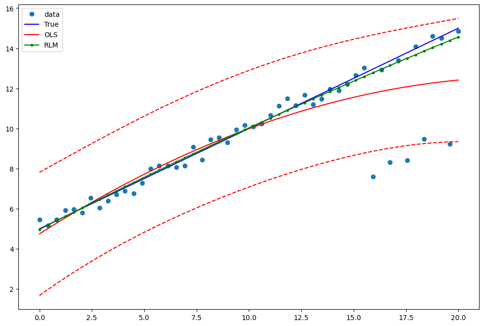
示例1:具有线性真实值的二次函数
请注意,OLS回归中的二次项将捕捉异常值效应。
[8]:
res = sm.OLS(y2, X).fit()
print(res.params)
print(res.bse)
print(res.predict())
[ 5.09508929  0.5244483  -0.01408909]
[0.47199871 0.07287023 0.00644789]
[ 4.74286192  5.01208175  5.27660718  5.5364382   5.7915748   6.042017
  6.28776479  6.52881817  6.76517714  6.9968417   7.22381186  7.4460876
  7.66366894  7.87655586  8.08474838  8.28824649  8.48705019  8.68115948
  8.87057436  9.05529484  9.2353209   9.41065256  9.5812898   9.74723264
  9.90848107 10.06503509 10.2168947  10.3640599  10.50653069 10.64430708
 10.77738905 10.90577662 11.02946978 11.14846853 11.26277287 11.3723828
 11.47729832 11.57751943 11.67304613 11.76387843 11.85001632 11.93145979
 12.00820886 12.08026352 12.14762377 12.21028961 12.26826104 12.32153807
 12.37012068 12.41400889]
估计 RLM:
[9]:
resrlm = sm.RLM(y2, X).fit()
print(resrlm.params)
print(resrlm.bse)
[ 5.03229730e+00  5.06226669e-01 -2.65264062e-03]
[0.1343856  0.02074732 0.00183582]
绘制一个图表以比较OLS估计与稳健估计:
[10]:
fig = plt.figure(figsize=(12, 8))
ax = fig.add_subplot(111)
ax.plot(x1, y2, "o", label="data")
ax.plot(x1, y_true2, "b-", label="True")
pred_ols = res.get_prediction()
iv_l = pred_ols.summary_frame()["obs_ci_lower"]
iv_u = pred_ols.summary_frame()["obs_ci_upper"]

ax.plot(x1, res.fittedvalues, "r-", label="OLS")
ax.plot(x1, iv_u, "r--")
ax.plot(x1, iv_l, "r--")
ax.plot(x1, resrlm.fittedvalues, "g.-", label="RLM")
ax.legend(loc="best")
[10]:
<matplotlib.legend.Legend at 0x119515590>
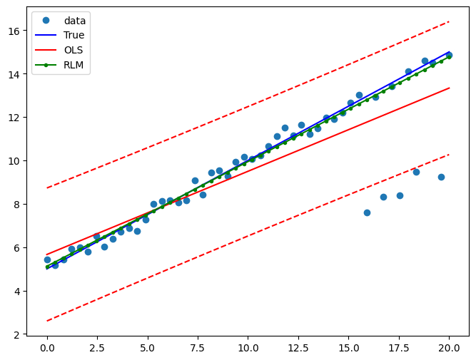
示例 2: 线性函数与线性真实值
使用仅包含线性项和常数项拟合一个新的OLS模型:
[11]:
X2 = X[:, [0, 1]]
res2 = sm.OLS(y2, X2).fit()
print(res2.params)
print(res2.bse)
[5.66296607 0.38355735]
[0.40920378 0.03525865]
估计 RLM:
[12]:
resrlm2 = sm.RLM(y2, X2).fit()
print(resrlm2.params)
print(resrlm2.bse)
[5.12061071 0.48269995]
[0.10345879 0.00891443]
绘制一个图表以比较OLS估计与稳健估计:
[13]:
pred_ols = res2.get_prediction()
iv_l = pred_ols.summary_frame()["obs_ci_lower"]
iv_u = pred_ols.summary_frame()["obs_ci_upper"]

fig, ax = plt.subplots(figsize=(8, 6))
ax.plot(x1, y2, "o", label="data")
ax.plot(x1, y_true2, "b-", label="True")
ax.plot(x1, res2.fittedvalues, "r-", label="OLS")
ax.plot(x1, iv_u, "r--")
ax.plot(x1, iv_l, "r--")
ax.plot(x1, resrlm2.fittedvalues, "g.-", label="RLM")
legend = ax.legend(loc="best")
Last update:
Oct 16, 2024