Theta 模型
Assimakopoulos & Nikolopoulos (2000) 的 Theta 模型是一种简单的预测方法,涉及拟合两条 \(\theta\)-线,使用简单指数平滑法对这两条线进行预测,然后将两条线的预测结果结合起来,生成最终的预测。该模型的实现步骤如下:
测试季节性
如果检测到季节性,则进行去季节化处理
通过将SES模型拟合到数据来估计\(\alpha\),并通过OLS估计\(b_0\)。
预测序列
如果数据已经去季节性化,请重新季节性化。
季节性检验检查季节性滞后 \(m\) 处的自相关函数(ACF)。如果该滞后显著不同于零,则使用 statsmodels.tsa.seasonal_decompose 对数据进行去季节化处理,使用乘法方法(默认)或加法方法。
模型的参数是 \(b_0\) 和 \(\alpha\),其中 \(b_0\) 是从OLS回归中估计出来的
并且 \(\alpha\) 是 SES 平滑参数
预测结果如下
最终,\(\theta\) 仅在确定趋势被抑制的程度时起作用。如果 \(\theta\) 非常大,那么模型的预测与带有漂移的积分移动平均值的预测相同。
最后,如果需要,预测结果会被重新季节性调整。
此模块基于:
Assimakopoulos, V., & Nikolopoulos, K. (2000). The theta 模型:一种分解预测方法。国际预测杂志, 16(4), 521-530.
Hyndman, R. J., & Billah, B. (2003). 揭开Theta方法的面纱。国际预测杂志, 19(2), 287-290.
Fioruci, J. A., Pellegrini, T. R., Louzada, F., & Petropoulos, F. (2015). 优化的theta方法。arXiv预印本 arXiv:1503.03529。
导入
我们从标准的导入集开始,并对默认的matplotlib样式进行一些调整。
[1]:
import matplotlib.pyplot as plt
import numpy as np
import pandas as pd
import pandas_datareader as pdr
import seaborn as sns

plt.rc("figure", figsize=(16, 8))
plt.rc("font", size=15)
plt.rc("lines", linewidth=3)
sns.set_style("darkgrid")
加载一些数据
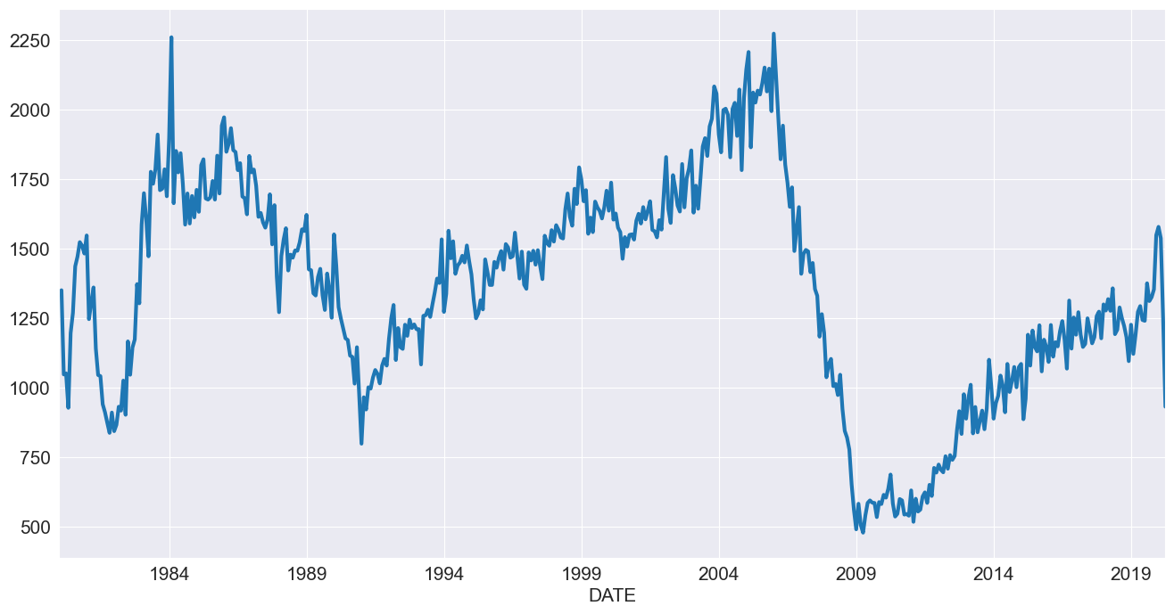
我们将首先使用美国数据来观察房屋开工情况。这一系列数据显然具有季节性,但在同一时期内并没有明显的趋势。
[2]:
reader = pdr.fred.FredReader(["HOUST"], start="1980-01-01", end="2020-04-01")
data = reader.read()
housing = data.HOUST
housing.index.freq = housing.index.inferred_freq
ax = housing.plot()
我们拟合了没有任何选项的模型并进行了拟合。摘要显示数据使用了乘法方法进行了去季节化处理。漂移是适度的且为负值,平滑参数相当低。
[3]:
from statsmodels.tsa.forecasting.theta import ThetaModel

tm = ThetaModel(housing)
res = tm.fit()
print(res.summary())
                              ThetaModel Results
==============================================================================
Dep. Variable:                  HOUST   No. Observations:                  484
Method:                       OLS/SES   Deseasonalized:                   True
Date:                Wed, 16 Oct 2024   Deseas. Method:         Multiplicative
Time:                        18:27:39   Period:                             12
Sample:                    01-01-1980
                         - 04-01-2020
   Parameter Estimates
=========================
           Parameters
-------------------------
b0    -0.9194460961668148
alpha   0.616996789006705
-------------------------
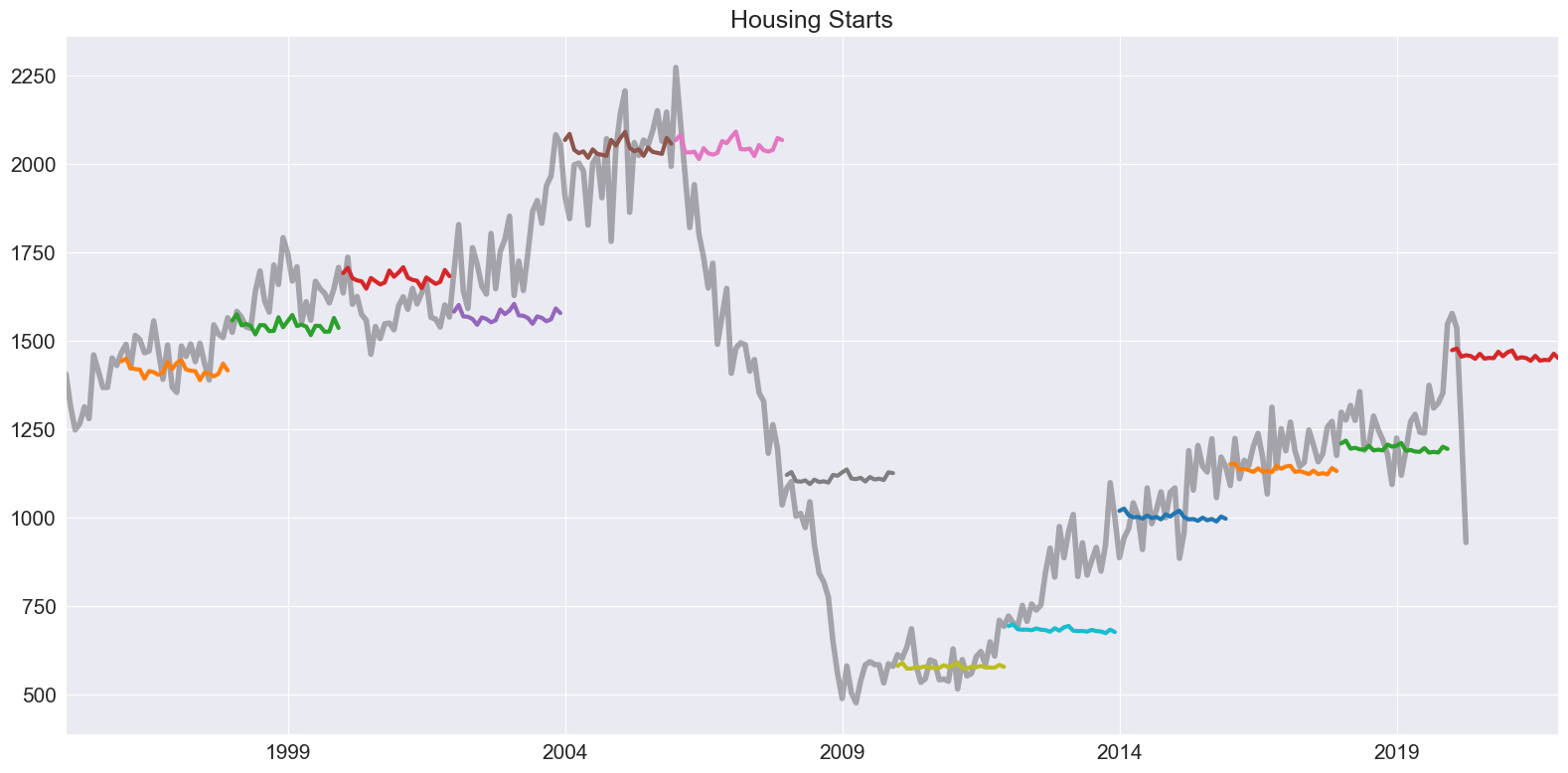
该模型首先是一种预测方法。使用拟合模型中的 forecast 方法生成预测。下面我们通过每两年预测未来两年生成一个刺猬图。
注意:默认的 \(\theta\) 是 2。
[4]:
forecasts = {"housing": housing}
for year in range(1995, 2020, 2):
    sub = housing[: str(year)]
    res = ThetaModel(sub).fit()
    fcast = res.forecast(24)
    forecasts[str(year)] = fcast
forecasts = pd.DataFrame(forecasts)
ax = forecasts["1995":].plot(legend=False)
children = ax.get_children()
children[0].set_linewidth(4)
children[0].set_alpha(0.3)
children[0].set_color("#000000")
ax.set_title("Housing Starts")
plt.tight_layout(pad=1.0)
我们可以选择拟合数据的自然对数。在这里,如果需要,强制使用加法方法进行去季节化更有意义。我们还使用最大似然估计(MLE)来拟合模型参数。这种方法拟合IMA
其中 \(\hat{\alpha}\) = \(\min(\hat{\gamma}+1, 0.9998)\) 使用 statsmodels.tsa.SARIMAX。参数相似,尽管漂移更接近于零。
[5]:
tm = ThetaModel(np.log(housing), method="additive")
res = tm.fit(use_mle=True)
print(res.summary())
                              ThetaModel Results
==============================================================================
Dep. Variable:                  HOUST   No. Observations:                  484
Method:                           MLE   Deseasonalized:                   True
Date:                Wed, 16 Oct 2024   Deseas. Method:               Additive
Time:                        18:27:40   Period:                             12
Sample:                    01-01-1980
                         - 04-01-2020
     Parameter Estimates
=============================
             Parameters
-----------------------------
b0    -0.00044644118699158845
alpha      0.6706103849698464
-----------------------------
预测仅取决于预测趋势成分,
来自SES的预测(不随时间范围变化),以及季节性。这三个组成部分可以通过forecast_components获得。这使得可以使用上述权重表达式,通过多种\(\theta\)选择来构建预测。
[6]:
res.forecast_components(12)
[6]:
| trend | ses | seasonal | |
|---|---|---|---|
| 2020-05-01 | -0.000666 | 6.95726 | -0.001252 |
| 2020-06-01 | -0.001112 | 6.95726 | -0.006891 |
| 2020-07-01 | -0.001559 | 6.95726 | 0.002992 |
| 2020-08-01 | -0.002005 | 6.95726 | -0.003817 |
| 2020-09-01 | -0.002451 | 6.95726 | -0.003902 |
| 2020-10-01 | -0.002898 | 6.95726 | -0.003981 |
| 2020-11-01 | -0.003344 | 6.95726 | 0.008536 |
| 2020-12-01 | -0.003791 | 6.95726 | -0.000714 |
| 2021-01-01 | -0.004237 | 6.95726 | 0.005239 |
| 2021-02-01 | -0.004684 | 6.95726 | 0.009943 |
| 2021-03-01 | -0.005130 | 6.95726 | -0.004535 |
| 2021-04-01 | -0.005577 | 6.95726 | -0.001619 |
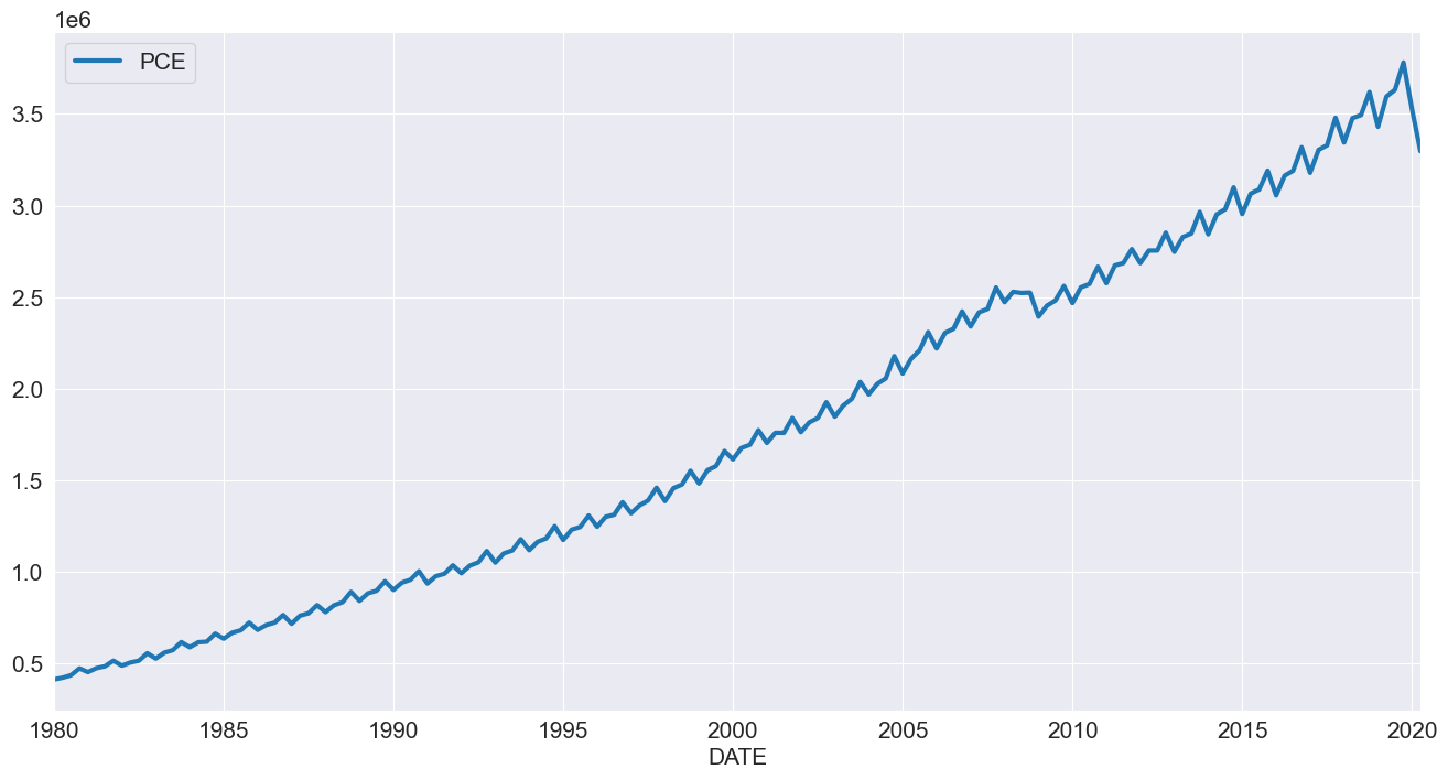
个人消费支出
我们接下来考察个人消费支出。这一系列数据具有明显的季节性成分和趋势。
[7]:
reader = pdr.fred.FredReader(["NA000349Q"], start="1980-01-01", end="2020-04-01")
pce = reader.read()
pce.columns = ["PCE"]
pce.index.freq = "QS-OCT"
_ = pce.plot()
由于这个序列总是正的,我们对该序列进行\(\ln\)建模。
[8]:
mod = ThetaModel(np.log(pce))
res = mod.fit()
print(res.summary())
                              ThetaModel Results
==============================================================================
Dep. Variable:                    PCE   No. Observations:                  162
Method:                       OLS/SES   Deseasonalized:                   True
Date:                Wed, 16 Oct 2024   Deseas. Method:         Multiplicative
Time:                        18:27:42   Period:                              4
Sample:                    01-01-1980
                         - 04-01-2020
   Parameter Estimates
==========================
           Parameters
--------------------------
b0    0.013035370221488499
alpha   0.9998851279204637
--------------------------
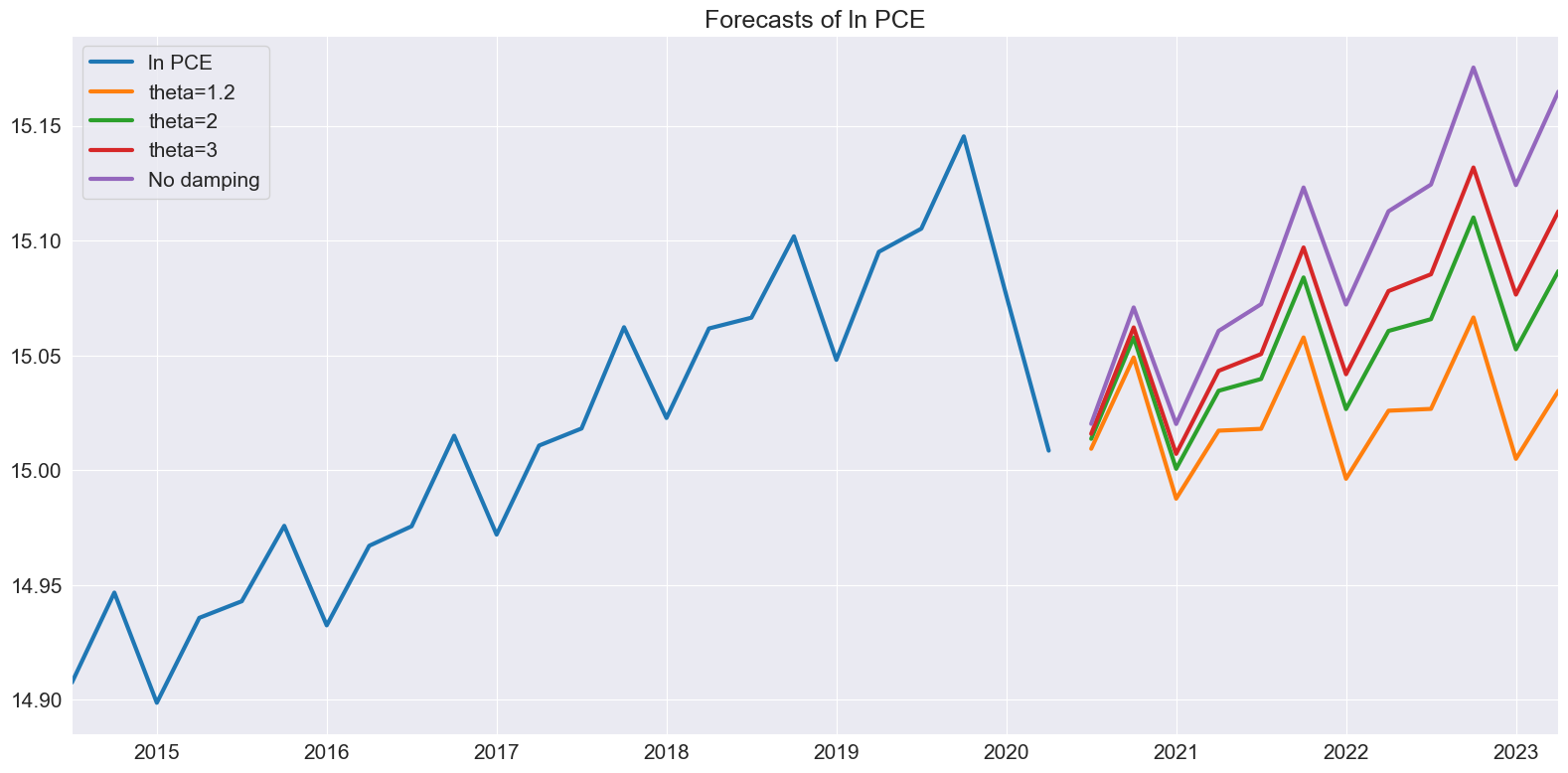
接下来我们探讨随着 \(\theta\) 的变化,预测中的差异。当 \(\theta\) 接近1时,漂移几乎不存在。随着 \(\theta\) 的增加,漂移变得更加明显。
[9]:
forecasts = pd.DataFrame(
    {
        "ln PCE": np.log(pce.PCE),
        "theta=1.2": res.forecast(12, theta=1.2),
        "theta=2": res.forecast(12),
        "theta=3": res.forecast(12, theta=3),
        "No damping": res.forecast(12, theta=np.inf),
    }
)
_ = forecasts.tail(36).plot()
plt.title("Forecasts of ln PCE")
plt.tight_layout(pad=1.0)
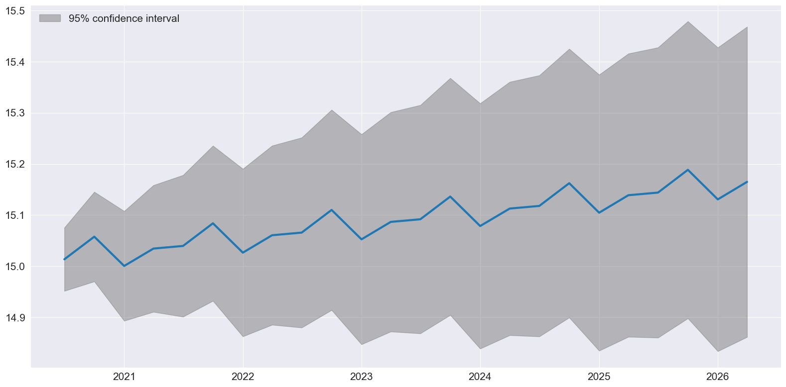
最后,plot_predict 可以用于可视化预测和预测区间,这些预测和预测区间是假设IMA为真的情况下构建的。
[10]:
ax = res.plot_predict(24, theta=2)
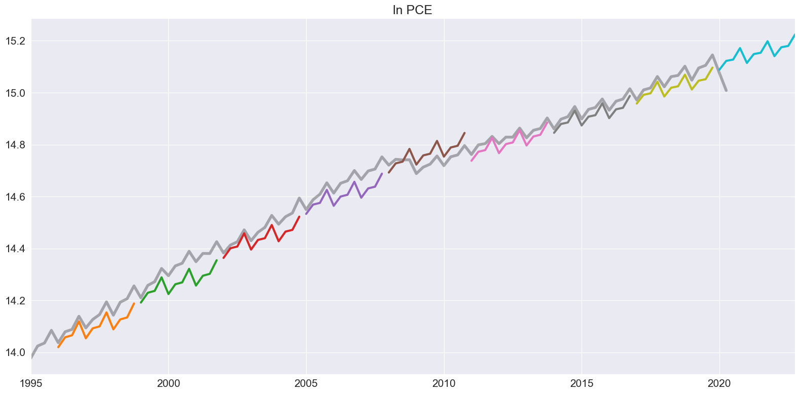
我们通过使用2年非重叠样本来生成刺猬图。
[11]:
ln_pce = np.log(pce.PCE)
forecasts = {"ln PCE": ln_pce}
for year in range(1995, 2020, 3):
    sub = ln_pce[: str(year)]
    res = ThetaModel(sub).fit()
    fcast = res.forecast(12)
    forecasts[str(year)] = fcast
forecasts = pd.DataFrame(forecasts)
ax = forecasts["1995":].plot(legend=False)
children = ax.get_children()
children[0].set_linewidth(4)
children[0].set_alpha(0.3)
children[0].set_color("#000000")
ax.set_title("ln PCE")
plt.tight_layout(pad=1.0)