生存和持续时间分析方法
statsmodels.duration 实现了几种处理删失数据的标准方法。这些方法最常用于数据由起始时间点到感兴趣事件发生时间之间的时间段组成的情况。一个典型的例子是医学研究,其中起始时间是某个受试者被诊断出某种疾病的时间,而感兴趣的事件是死亡(或疾病进展、康复等)。
目前仅处理右删失。右删失发生在当我们知道某个事件在给定时间t之后发生,但我们不知道确切的事件时间。
生存函数估计与推断
statsmodels.api.SurvfuncRight 类可用于使用可能存在右删失的数据估计生存函数。
SurvfuncRight 实现了几种推理程序,包括生存分布分位数的置信区间、生存函数的逐点置信带和同时置信带,以及绘图程序。duration.survdiff 函数提供了比较生存分布的检验程序。
这里我们使用来自flchain研究的数据创建一个SurvfuncRight对象,该研究可通过R数据集仓库获得。我们仅对女性受试者拟合生存分布。
In [1]: import statsmodels.api as sm

In [2]: data = sm.datasets.get_rdataset("flchain", "survival").data

In [3]: df = data.loc[data.sex == "F", :]

In [4]: sf = sm.SurvfuncRight(df["futime"], df["death"])
通过调用summary方法,可以查看拟合生存分布的主要特征:
In [5]: sf.summary().head()
Out[5]:
      Surv prob  Surv prob SE  num at risk  num events
Time
0      0.999310      0.000398         4350         3.0
1      0.998851      0.000514         4347         2.0
2      0.998621      0.000563         4343         1.0
3      0.997931      0.000689         4342         3.0
4      0.997471      0.000762         4338         2.0
我们可以获得生存分布分位数的点估计和置信区间。由于在这项研究中只有大约30%的受试者死亡,我们只能估计低于0.3概率点的分位数:
In [6]: sf.quantile(0.25)
Out[6]: np.int64(3995)

In [7]: sf.quantile_ci(0.25)
Out[7]: (np.int64(3776), np.int64(4166))
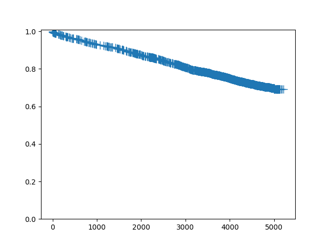
要绘制单个生存函数,请调用plot方法:
In [8]: sf.plot()
Out[8]: <Figure size 640x480 with 1 Axes>
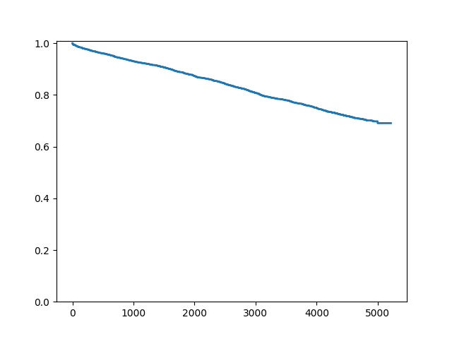
由于这是一个包含大量审查的大数据集,我们可能希望不绘制审查符号:
In [9]: fig = sf.plot()

In [10]: ax = fig.get_axes()[0]

In [11]: pt = ax.get_lines()[1]

In [12]: pt.set_visible(False)
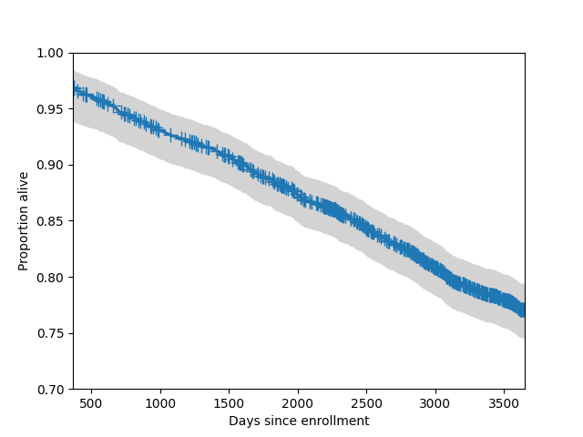
我们还可以在图中添加一个95%的同时置信带。 通常这些带仅绘制在分布的中心部分。
In [13]: fig = sf.plot()

In [14]: lcb, ucb = sf.simultaneous_cb()

In [15]: ax = fig.get_axes()[0]

In [16]: ax.fill_between(sf.surv_times, lcb, ucb, color='lightgrey')
Out[16]: <matplotlib.collections.PolyCollection at 0x12a585e90>

In [17]: ax.set_xlim(365, 365*10)
Out[17]: (365.0, 3650.0)

In [18]: ax.set_ylim(0.7, 1)
Out[18]: (0.7, 1.0)

In [19]: ax.set_ylabel("Proportion alive")
Out[19]: Text(0, 0.5, 'Proportion alive')

In [20]: ax.set_xlabel("Days since enrollment")
Out[20]: Text(0.5, 0, 'Days since enrollment')
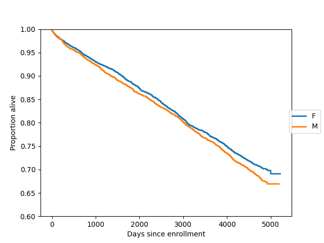
这里我们在同一坐标轴上绘制了两个组(女性和男性)的生存函数:
In [21]: import matplotlib.pyplot as plt

In [22]: gb = data.groupby("sex")

In [23]: ax = plt.axes()

In [24]: sexes = []

In [25]: for g in gb:
   ....:     sexes.append(g[0])
   ....:     sf = sm.SurvfuncRight(g[1]["futime"], g[1]["death"])
   ....:     sf.plot(ax)
   ....:

In [26]: li = ax.get_lines()

In [27]: li[1].set_visible(False)

In [28]: li[3].set_visible(False)

In [29]: plt.figlegend((li[0], li[2]), sexes, loc="center right")
Out[29]: <matplotlib.legend.Legend at 0x12affaf10>

In [30]: plt.ylim(0.6, 1)
Out[30]: (0.6, 1.0)

In [31]: ax.set_ylabel("Proportion alive")
Out[31]: Text(0, 0.5, 'Proportion alive')

In [32]: ax.set_xlabel("Days since enrollment")
Out[32]: Text(0.5, 0, 'Days since enrollment')
我们可以使用survdiff正式比较两个生存分布,它实现了几种标准的非参数程序。默认程序是对数秩检验:
In [33]: stat, pv = sm.duration.survdiff(data.futime, data.death, data.sex)
以下是survdiff实现的一些其他测试程序:
 # Fleming-Harrington with p=1, i.e. weight by pooled survival time
In [34]: stat, pv = sm.duration.survdiff(data.futime, data.death, data.sex, weight_type='fh', fh_p=1)

 # Gehan-Breslow, weight by number at risk
In [35]: stat, pv = sm.duration.survdiff(data.futime, data.death, data.sex, weight_type='gb')

 # Tarone-Ware, weight by the square root of the number at risk
In [36]: stat, pv = sm.duration.survdiff(data.futime, data.death, data.sex, weight_type='tw')
回归方法
比例风险回归模型(“Cox模型”)是一种用于截尾数据的回归技术。它们允许事件发生时间的变化通过协变量来解释,类似于在线性或广义线性回归模型中所做的那样。这些模型通过“风险比”来表达协变量的影响,这意味着风险(瞬时事件率)会根据协变量的值乘以一个给定的因子。
In [37]: import statsmodels.api as sm

In [38]: import statsmodels.formula.api as smf

In [39]: data = sm.datasets.get_rdataset("flchain", "survival").data

In [40]: del data["chapter"]

In [41]: data = data.dropna()

In [42]: data["lam"] = data["lambda"]

In [43]: data["female"] = (data["sex"] == "F").astype(int)

In [44]: data["year"] = data["sample.yr"] - min(data["sample.yr"])

In [45]: status = data["death"].values

In [46]: mod = smf.phreg("futime ~ 0 + age + female + creatinine + np.sqrt(kappa) + np.sqrt(lam) + year + mgus", data, status=status, ties="efron")

In [47]: rslt = mod.fit()

In [48]: print(rslt.summary())
                           Results: PHReg
====================================================================
Model:                      PH Reg         Sample size:         6524
Dependent variable:         futime         Num. events:         1962
Ties:                       Efron
--------------------------------------------------------------------
                log HR log HR SE   HR      t    P>|t|  [0.025 0.975]
--------------------------------------------------------------------
age             0.1012    0.0025 1.1065 40.9289 0.0000 1.1012 1.1119
female         -0.2817    0.0474 0.7545 -5.9368 0.0000 0.6875 0.8280
creatinine      0.0134    0.0411 1.0135  0.3271 0.7436 0.9351 1.0985
np.sqrt(kappa)  0.4047    0.1147 1.4988  3.5288 0.0004 1.1971 1.8766
np.sqrt(lam)    0.7046    0.1117 2.0230  6.3056 0.0000 1.6251 2.5183
year            0.0477    0.0192 1.0489  2.4902 0.0128 1.0102 1.0890
mgus            0.3160    0.2532 1.3717  1.2479 0.2121 0.8350 2.2532
====================================================================
Confidence intervals are for the hazard ratios
参见示例以获取更详细的示例。
Wiki上有一些笔记本示例: PHReg和生存分析的Wiki笔记本
参考文献
Cox比例风险回归模型的参考资料:
T Therneau (1996). Extending the Cox model. Technical report.
http://www.mayo.edu/research/documents/biostat-58pdf/DOC-10027288

G Rodriguez (2005). Non-parametric estimation in survival models.
http://data.princeton.edu/pop509/NonParametricSurvival.pdf

B Gillespie (2006). Checking the assumptions in the Cox proportional
hazards model.
http://www.mwsug.org/proceedings/2006/stats/MWSUG-2006-SD08.pdf
模块参考
用于处理生存分布的类是:
|
生存函数的估计和推断。 |
比例风险回归模型类是:
|
Cox比例风险回归模型 |
比例风险回归结果类是:
|
包含拟合Cox比例风险生存模型结果的类。 |
主要的辅助类是:
|
一个表示离散分布集合的类。 |