时间序列过滤器
[1]:
%matplotlib inline
[2]:
import pandas as pd
import matplotlib.pyplot as plt

import statsmodels.api as sm
[3]:
dta = sm.datasets.macrodata.load_pandas().data
[4]:
index = pd.Index(sm.tsa.datetools.dates_from_range("1959Q1", "2009Q3"))
print(index)
DatetimeIndex(['1959-03-31', '1959-06-30', '1959-09-30', '1959-12-31',
               '1960-03-31', '1960-06-30', '1960-09-30', '1960-12-31',
               '1961-03-31', '1961-06-30',
               ...
               '2007-06-30', '2007-09-30', '2007-12-31', '2008-03-31',
               '2008-06-30', '2008-09-30', '2008-12-31', '2009-03-31',
               '2009-06-30', '2009-09-30'],
              dtype='datetime64[ns]', length=203, freq=None)
[5]:
dta.index = index
del dta["year"]
del dta["quarter"]
[6]:
print(sm.datasets.macrodata.NOTE)
::
    Number of Observations - 203

    Number of Variables - 14

    Variable name definitions::

        year      - 1959q1 - 2009q3
        quarter   - 1-4
        realgdp   - Real gross domestic product (Bil. of chained 2005 US$,
                    seasonally adjusted annual rate)
        realcons  - Real personal consumption expenditures (Bil. of chained
                    2005 US$, seasonally adjusted annual rate)
        realinv   - Real gross private domestic investment (Bil. of chained
                    2005 US$, seasonally adjusted annual rate)
        realgovt  - Real federal consumption expenditures & gross investment
                    (Bil. of chained 2005 US$, seasonally adjusted annual rate)
        realdpi   - Real private disposable income (Bil. of chained 2005
                    US$, seasonally adjusted annual rate)
        cpi       - End of the quarter consumer price index for all urban
                    consumers: all items (1982-84 = 100, seasonally adjusted).
        m1        - End of the quarter M1 nominal money stock (Seasonally
                    adjusted)
        tbilrate  - Quarterly monthly average of the monthly 3-month
                    treasury bill: secondary market rate
        unemp     - Seasonally adjusted unemployment rate (%)
        pop       - End of the quarter total population: all ages incl. armed
                    forces over seas
        infl      - Inflation rate (ln(cpi_{t}/cpi_{t-1}) * 400)
        realint   - Real interest rate (tbilrate - infl)
[7]:
print(dta.head(10))
             realgdp  realcons  realinv  realgovt  realdpi    cpi     m1  \
1959-03-31  2710.349    1707.4  286.898   470.045   1886.9  28.98  139.7
1959-06-30  2778.801    1733.7  310.859   481.301   1919.7  29.15  141.7
1959-09-30  2775.488    1751.8  289.226   491.260   1916.4  29.35  140.5
1959-12-31  2785.204    1753.7  299.356   484.052   1931.3  29.37  140.0
1960-03-31  2847.699    1770.5  331.722   462.199   1955.5  29.54  139.6
1960-06-30  2834.390    1792.9  298.152   460.400   1966.1  29.55  140.2
1960-09-30  2839.022    1785.8  296.375   474.676   1967.8  29.75  140.9
1960-12-31  2802.616    1788.2  259.764   476.434   1966.6  29.84  141.1
1961-03-31  2819.264    1787.7  266.405   475.854   1984.5  29.81  142.1
1961-06-30  2872.005    1814.3  286.246   480.328   2014.4  29.92  142.9

            tbilrate  unemp      pop  infl  realint
1959-03-31      2.82    5.8  177.146  0.00     0.00
1959-06-30      3.08    5.1  177.830  2.34     0.74
1959-09-30      3.82    5.3  178.657  2.74     1.09
1959-12-31      4.33    5.6  179.386  0.27     4.06
1960-03-31      3.50    5.2  180.007  2.31     1.19
1960-06-30      2.68    5.2  180.671  0.14     2.55
1960-09-30      2.36    5.6  181.528  2.70    -0.34
1960-12-31      2.29    6.3  182.287  1.21     1.08
1961-03-31      2.37    6.8  182.992 -0.40     2.77
1961-06-30      2.29    7.0  183.691  1.47     0.81
[8]:
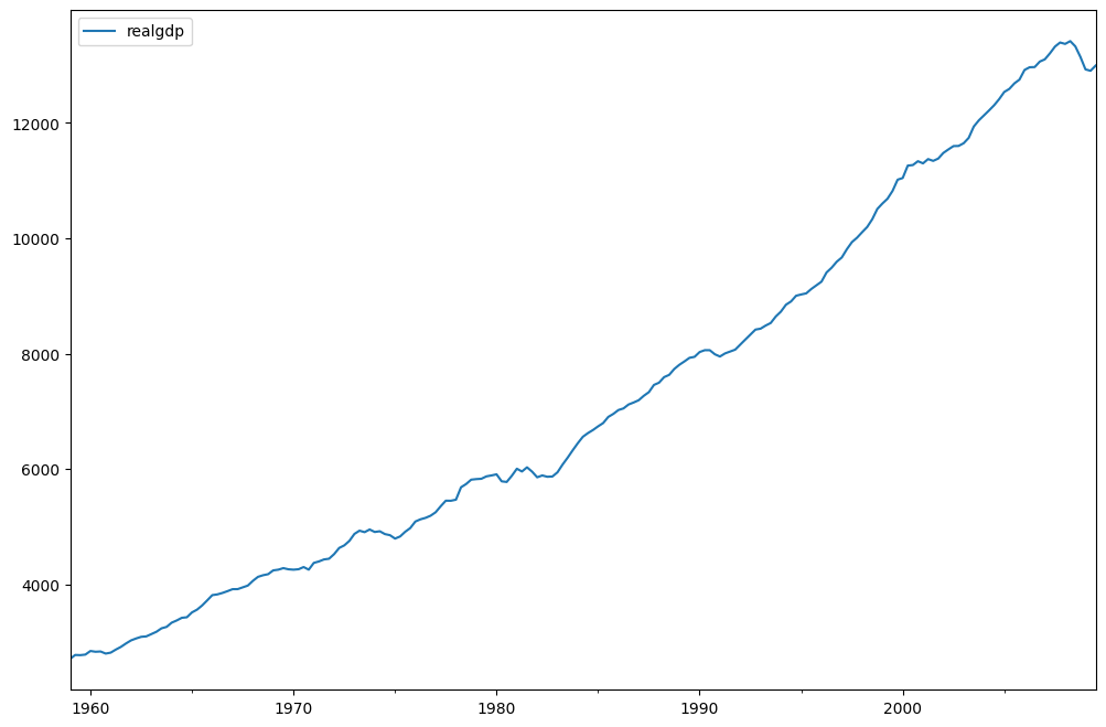
fig = plt.figure(figsize=(12, 8))
ax = fig.add_subplot(111)
dta.realgdp.plot(ax=ax)
legend = ax.legend(loc="upper left")
legend.prop.set_size(20)
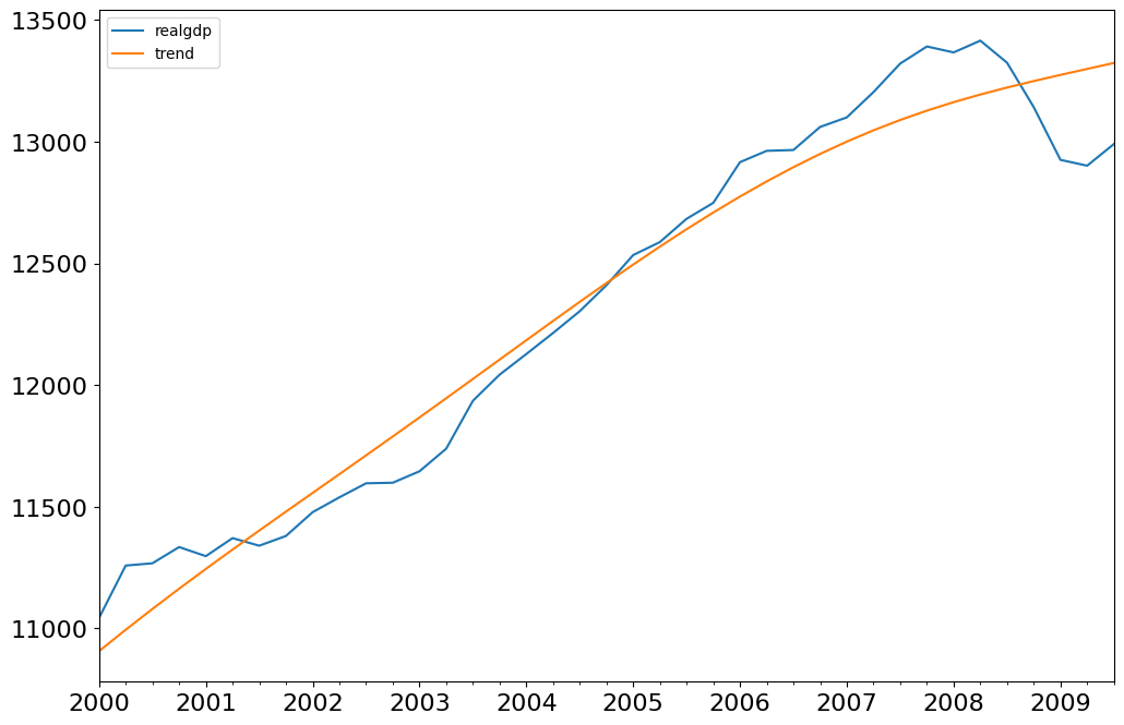
Hodrick-Prescott 滤波器
Hodrick-Prescott滤波器将时间序列\(y_t\)分解为趋势\(\tau_t\)和周期性成分\(\zeta_t\)
通过最小化以下二次损失函数来确定组件
[9]:
gdp_cycle, gdp_trend = sm.tsa.filters.hpfilter(dta.realgdp)
[10]:
gdp_decomp = dta[["realgdp"]].copy()
gdp_decomp["cycle"] = gdp_cycle
gdp_decomp["trend"] = gdp_trend
[11]:
fig = plt.figure(figsize=(12, 8))
ax = fig.add_subplot(111)
gdp_decomp[["realgdp", "trend"]]["2000-03-31":].plot(ax=ax, fontsize=16)
legend = ax.get_legend()
legend.prop.set_size(20)
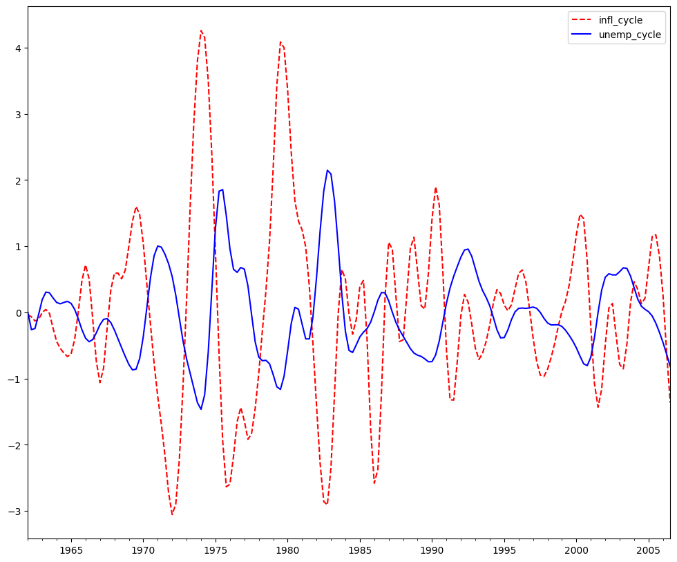
Baxter-King近似带通滤波器: 通货膨胀和失业
探讨通货膨胀和失业率呈反周期性的假设。
Baxter-King 滤波器旨在明确处理商业周期的周期性。通过将他们的带通滤波器应用于一个序列,他们生成一个不包含高于或低于商业周期波动的新序列。具体来说,BK 滤波器采用对称移动平均的形式
其中 \(a_{-k}=a_k\) 且 \(\sum_{k=-k}^{K}a_k=0\) 以消除序列中的任何趋势,并使其平稳,如果序列是 I(1) 或 I(2)。
为了完整性,过滤器权重确定如下
其中 \(\theta\) 是一个归一化常数,使得权重之和为零。
\(P_L\) 和 \(P_H\) 是低和高截止频率的周期性。根据Burns和Mitchell关于美国商业周期的研究,建议周期持续时间为1.5到8年,我们默认使用 \(P_L=6\) 和 \(P_H=32\)。
[12]:
bk_cycles = sm.tsa.filters.bkfilter(dta[["infl", "unemp"]])
我们在两端丢失了K个观测值。建议对季度数据使用K=12。
[13]:
fig = plt.figure(figsize=(12, 10))
ax = fig.add_subplot(111)
bk_cycles.plot(ax=ax, style=["r--", "b-"])
[13]:
<Axes: >
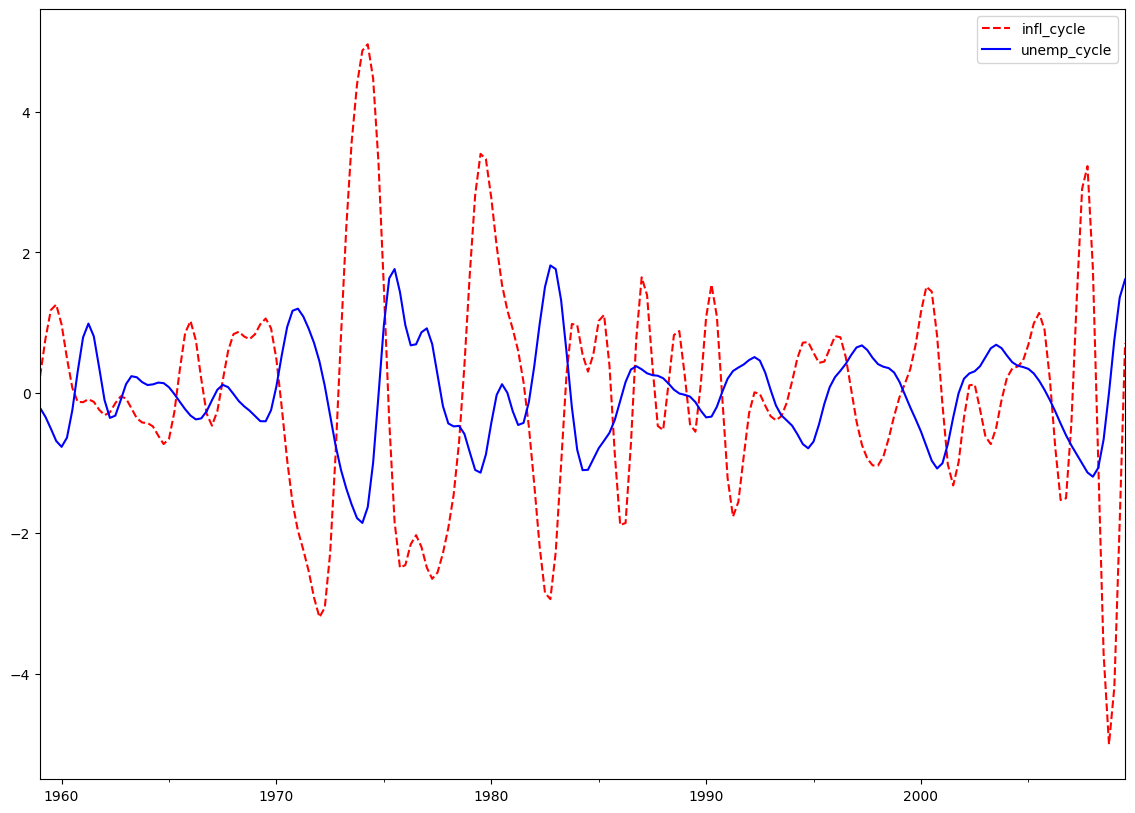
Christiano-Fitzgerald 近似带通滤波器: 通货膨胀和失业
Christiano-Fitzgerald 滤波器是 BK 的泛化,因此也可以被视为加权移动平均。然而,CF 滤波器在 \(t\) 处是不对称的,并且使用了整个序列。他们的滤波器的实现涉及在
对于 \(t=3,4,...,T-2\),其中
\(\tilde B_{T-t}\) 和 \(\tilde B_{t-1}\) 是 \(B_{j}\) 的线性函数,并且 \(t=1,2,T-1,\) 和 \(T\) 的值也是以类似的方式计算的。\(P_{U}\) 和 \(P_{L}\) 如上所述,具有相同的解释。
CF 滤波器适用于可能遵循随机游走的序列。
[14]:
print(sm.tsa.stattools.adfuller(dta["unemp"])[:3])
(np.float64(-2.5364584673346355), np.float64(0.10685366457233497), 9)
[15]:
print(sm.tsa.stattools.adfuller(dta["infl"])[:3])
(np.float64(-3.054514496257235), np.float64(0.030107620863486003), 2)
[16]:
cf_cycles, cf_trend = sm.tsa.filters.cffilter(dta[["infl", "unemp"]])
print(cf_cycles.head(10))
            infl_cycle  unemp_cycle
1959-03-31    0.237927    -0.216867
1959-06-30    0.770007    -0.343779
1959-09-30    1.177736    -0.511024
1959-12-31    1.256754    -0.686967
1960-03-31    0.972128    -0.770793
1960-06-30    0.491889    -0.640601
1960-09-30    0.070189    -0.249741
1960-12-31   -0.130432     0.301545
1961-03-31   -0.134155     0.788992
1961-06-30   -0.092073     0.985356
[17]:
fig = plt.figure(figsize=(14, 10))
ax = fig.add_subplot(111)
cf_cycles.plot(ax=ax, style=["r--", "b-"])
[17]:
<Axes: >
过滤假设先验存在商业周期。由于这一假设,许多宏观经济模型试图创建与脉冲响应函数形状相匹配的模型,而不是复制过滤序列的属性。请参阅VAR笔记本。