
过去十年著名演讲的情感分析#
小心
本文目前未经过测试。帮助改进本教程,使其完全可执行!
本教程演示了如何使用 NumPy 从头构建一个简单的 长短期记忆网络 (LSTM) 来对一个与社会相关且伦理上获取的数据集进行情感分析。
你的深度学习模型(LSTM)是一种循环神经网络的形式,将从IMDB评论数据集中学习将一段文本分类为正面或负面。该数据集包含50,000条电影评论及其相应的标签。基于这些评论的数值表示及其相应标签 (监督学习),神经网络将通过前向传播和时间反向传播进行训练,以学习情感,因为我们在这里处理的是序列数据。输出将是一个包含文本样本为正面概率的向量。
今天,深度学习正被日常生活中的应用所采用,现在确保使用人工智能做出的决策不会对某一群体表现出歧视行为更为重要。在消费人工智能的输出时,考虑公平性是重要的。在整个教程中,我们将尝试从伦理的角度质疑我们管道中的所有步骤。
前提条件#
你需要熟悉Python编程语言和使用NumPy进行数组操作。此外,建议对线性代数和微积分有一定的了解。你还应该熟悉神经网络的工作原理。你可以访问Python、线性代数在n维数组上的应用和微积分教程以供参考。
要复习深度学习基础知识,你应该考虑阅读 d2l.ai 书籍,这是一本带有多框架代码、数学和讨论的互动深度学习书籍。你也可以通过 从头开始在 MNIST 上进行深度学习教程 来理解如何从头实现一个基本的神经网络。
除了NumPy之外,您还将使用以下Python标准模块进行数据加载和处理:
pandas用于处理数据帧Matplotlib用于数据可视化pooch下载和缓存数据集
本教程可以在一个隔离的环境中本地运行,例如 Virtualenv 或 conda。你可以使用 Jupyter Notebook 或 JupyterLab 来运行每个笔记本单元。
目录#
数据收集
预处理数据集
从头开始构建和训练一个 LSTM 网络
对收集的演讲进行情感分析
下一步
1. Data Collection#
在开始之前,有几点你应该始终牢记在选择你要训练模型的数据之前:
识别数据偏差 - 偏差是人类思维过程的固有组成部分。因此,源自人类活动的数据反映了这种偏差。这种偏差在机器学习数据集中倾向于出现的一些方式有:
历史数据中的偏见:历史数据往往对特定群体有偏见,或者偏向于、或者反对特定群体。数据也可能严重不平衡,对受保护群体的信息有限。
数据收集机制中的偏差:缺乏代表性会在数据收集过程中引入固有的偏差。
偏向于可观察的结果:在某些情况下,我们只有关于部分人口的真实结果信息。在没有所有结果信息的情况下,甚至无法衡量公平性
保护敏感数据的个人匿名性:Trevisan 和 Reilly 确定了一系列需要特别小心处理的敏感话题。我们在下面列出了相同的内容,并增加了一些内容:
个人日常例行活动(包括位置数据);
关于损伤和/或医疗记录的个别细节;
疼痛和慢性疾病的情感描述;
关于收入和/或福利支付的财务信息;
歧视和虐待事件;
对个别医疗和支持服务提供者的批评/赞扬;
自杀念头;
对权力结构的批评/赞扬,特别是如果它危及他们的安全;
个人身份信息(即使以某种方式匿名化),包括指纹或声音等。
虽然从这么多人那里获取同意尤其在在线平台上可能很困难,但这种必要性取决于您的数据所包含主题的敏感性以及其他指标,例如数据来源的平台是否允许用户使用假名操作。如果网站有强制使用真实姓名的政策,那么需要征求用户的同意。
在本节中,您将收集两个不同的数据集:IMDb 电影评论数据集,以及为本教程精选的 10 篇演讲集,包括来自世界各地、不同时期和不同主题的活动家的演讲。前者将用于训练深度学习模型,而后者将用于进行情感分析。
收集 IMDb 评论数据集#
IMDb 评论数据集是一个大型电影评论数据集,由 Andrew L. Maas 从流行的电影评分服务 IMDb 收集和准备。IMDb 评论数据集用于二元情感分类,判断评论是正面还是负面。它包含 25,000 条用于训练的电影评论和 25,000 条用于测试的电影评论。所有这 50,000 条评论都是带标签的数据,可用于监督深度学习。为了便于复现,我们将从 Zenodo 获取数据。
IMDb 平台允许个人和非商业用途使用他们的公开数据集。我们尽力确保这些评论不包含任何上述与评论者相关的敏感话题。
收集和加载语音记录#
我们选择了来自全球活动家的演讲,讨论气候变化、女权主义、lgbtqa+权利和种族主义等问题。这些演讲来源于报纸、联合国官方网站和已建立的大学档案,如下表所引。创建了一个CSV文件,包含转录的演讲、演讲者和演讲来源。我们确保在数据中包含不同的人口统计数据,并涵盖了一系列不同的主题,其中大部分集中在社会和/或伦理问题上。
Speech |
Speaker |
源 |
|---|---|---|
Barnard 学院毕业典礼 |
莱玛·戈博韦 |
|
联合国关于青年教育的演讲 |
马拉拉·优素福扎伊 |
|
联合国大会关于种族歧视的讲话 |
琳达·托马斯·格林菲尔德 |
|
你好大胆 |
格蕾塔·桑伯格 |
|
那场让世界沉默了5分钟的演讲 |
塞文·铃木 |
|
希望演讲 |
哈维·米尔克 |
|
在Thrive会议上的演讲 |
艾伦·佩吉 |
|
我有一个梦想 |
马丁·路德·金 |
2. Preprocess the datasets#
数据预处理在构建任何深度学习模型之前是一个极其关键的步骤,然而为了保持教程专注于构建模型,我们将不会深入探讨预处理的代码。以下是我们为清理数据并将其转换为数值表示所采取的所有步骤的简要概述。
文本去噪 : 在将文本转换为向量之前,重要的是对其进行清理并去除所有无用的部分,即通过将所有字符转换为小写、去除html标签、括号和停用词(这些词对句子的意义贡献不大)来去除数据中的噪声。没有这一步,数据集通常是一堆计算机无法理解的词汇。
将单词转换为向量 : 词嵌入是一种学习的文本表示方法,其中具有相同含义的单词具有相似的表示。单个单词在预定义的向量空间中表示为实值向量。GloVe 是由斯坦福大学开发的无监督算法,通过从语料库生成全局词-词共现矩阵来生成词嵌入。您可以从 https://nlp.stanford.edu/projects/glove/ 下载包含嵌入的压缩文件。在这里,您可以选择四种不同大小或训练数据集的选项之一。我们选择了内存消耗最少的嵌入文件。
GloVe 词嵌入包括在数十亿个标记上训练的集合,有些甚至达到 8400 亿个标记。这些算法表现出典型的偏见,例如性别偏见,这可以追溯到原始训练数据。例如,某些职业似乎更偏向于特定性别,强化了有问题的刻板印象。解决这个问题的最接近方案是一些去偏算法,如 https://web.stanford.edu/class/archive/cs/cs224n/cs224n.1184/reports/6835575.pdf 中介绍的算法,人们可以在他们选择的嵌入上使用这些算法来缓解偏见,如果存在的话。
你将从导入必要的包开始构建我们的深度学习网络。
# Importing the necessary packages
import numpy as np
import pandas as pd
import matplotlib.pyplot as plt
import pooch
import string
import re
import zipfile
import os

# Creating the random instance
rng = np.random.default_rng()
接下来,您将定义一组文本预处理辅助函数。
class TextPreprocess:
    """Text Preprocessing for a Natural Language Processing model."""

    def txt_to_df(self, file):
        """Function to convert a txt file to pandas dataframe.

        Parameters
        ----------
        file : str
            Path to the txt file.

        Returns
        -------
        Pandas dataframe
            txt file converted to a dataframe.

        """
        with open(imdb_train, 'r') as in_file:
            stripped = (line.strip() for line in in_file)
            reviews = {}
            for line in stripped:
                lines = [splits for splits in line.split("\t") if splits != ""]
                reviews[lines[1]] = float(lines[0])
        df = pd.DataFrame(reviews.items(), columns=['review', 'sentiment'])
        df = df.sample(frac=1).reset_index(drop=True)
        return df

    def unzipper(self, zipped, to_extract):
        """Function to extract a file from a zipped folder.

        Parameters
        ----------
        zipped : str
            Path to the zipped folder.

        to_extract: str
            Path to the file to be extracted from the zipped folder

        Returns
        -------
        str
            Path to the extracted file.

        """
        fh = open(zipped, 'rb')
        z = zipfile.ZipFile(fh)
        outdir = os.path.split(zipped)[0]
        z.extract(to_extract, outdir)
        fh.close()
        output_file = os.path.join(outdir, to_extract)
        return output_file

    def cleantext(self, df, text_column=None,
                  remove_stopwords=True, remove_punc=True):
        """Function to clean text data.

        Parameters
        ----------
        df : pandas dataframe
            The dataframe housing the input data.
        text_column : str
            Column in dataframe whose text is to be cleaned.
        remove_stopwords : bool
            if True, remove stopwords from text
        remove_punc : bool
            if True, remove punctuation symbols from text

        Returns
        -------
        Numpy array
            Cleaned text.

        """
        # converting all characters to lowercase
        df[text_column] = df[text_column].str.lower()

        # List of stopwords taken from https://gist.github.com/sebleier/554280
        stopwords = ["a", "about", "above", "after", "again", "against",
                     "all", "am", "an", "and", "any", "are",
                     "as", "at", "be", "because",
                     "been", "before", "being", "below",
                     "between", "both", "but", "by", "could",
                     "did", "do", "does", "doing", "down", "during",
                     "each", "few", "for", "from", "further",
                     "had", "has", "have", "having", "he",
                     "he'd", "he'll", "he's", "her", "here",
                     "here's", "hers", "herself", "him",
                     "himself", "his", "how", "how's", "i",
                     "i'd", "i'll", "i'm", "i've",
                     "if", "in", "into",
                     "is", "it", "it's", "its",
                     "itself", "let's", "me", "more",
                     "most", "my", "myself", "nor", "of",
                     "on", "once", "only", "or",
                     "other", "ought", "our", "ours",
                     "ourselves", "out", "over", "own", "same",
                     "she", "she'd", "she'll", "she's", "should",
                     "so", "some", "such", "than", "that",
                     "that's", "the", "their", "theirs", "them",
                     "themselves", "then", "there", "there's",
                     "these", "they", "they'd", "they'll",
                     "they're", "they've", "this", "those",
                     "through", "to", "too", "under", "until", "up",
                     "very", "was", "we", "we'd", "we'll",
                     "we're", "we've", "were", "what",
                     "what's", "when", "when's",
                     "where", "where's",
                     "which", "while", "who", "who's",
                     "whom", "why", "why's", "with",
                     "would", "you", "you'd", "you'll",
                     "you're", "you've",
                     "your", "yours", "yourself", "yourselves"]

        def remove_stopwords(data, column):
            data[f'{column} without stopwords'] = data[column].apply(
                lambda x: ' '.join([word for word in x.split() if word not in (stopwords)]))
            return data

        def remove_tags(string):
            result = re.sub('<*>', '', string)
            return result

        # remove html tags and brackets from text
        if remove_stopwords:
            data_without_stopwords = remove_stopwords(df, text_column)
            data_without_stopwords[f'clean_{text_column}'] = data_without_stopwords[f'{text_column} without stopwords'].apply(
                lambda cw: remove_tags(cw))
        if remove_punc:
            data_without_stopwords[f'clean_{text_column}'] = data_without_stopwords[f'clean_{text_column}'].str.replace(
                '[{}]'.format(string.punctuation), ' ', regex=True)

        X = data_without_stopwords[f'clean_{text_column}'].to_numpy()

        return X


    def sent_tokeniser(self, x):
        """Function to split text into sentences.

        Parameters
        ----------
        x : str
            piece of text

        Returns
        -------
        list
            sentences with punctuation removed.

        """
        sentences = re.split(r'(?<!\w\.\w.)(?<![A-Z][a-z]\.)(?<=\.|\?)\s', x)
        sentences.pop()
        sentences_cleaned = [re.sub(r'[^\w\s]', '', x) for x in sentences]
        return sentences_cleaned

    def word_tokeniser(self, text):
        """Function to split text into tokens.

        Parameters
        ----------
        x : str
            piece of text

        Returns
        -------
        list
            words with punctuation removed.

        """
        tokens = re.split(r"([-\s.,;!?])+", text)
        words = [x for x in tokens if (
            x not in '- \t\n.,;!?\\' and '\\' not in x)]
        return words

    def loadGloveModel(self, emb_path):
        """Function to read from the word embedding file.

        Returns
        -------
        Dict
            mapping from word to corresponding word embedding.

        """
        print("Loading Glove Model")
        File = emb_path
        f = open(File, 'r')
        gloveModel = {}
        for line in f:
            splitLines = line.split()
            word = splitLines[0]
            wordEmbedding = np.array([float(value) for value in splitLines[1:]])
            gloveModel[word] = wordEmbedding
        print(len(gloveModel), " words loaded!")
        return gloveModel

    def text_to_paras(self, text, para_len):
        """Function to split text into paragraphs.

        Parameters
        ----------
        text : str
            piece of text

        para_len : int
            length of each paragraph

        Returns
        -------
        list
            paragraphs of specified length.

        """
        # split the speech into a list of words
        words = text.split()
        # obtain the total number of paragraphs
        no_paras = int(np.ceil(len(words)/para_len))
        # split the speech into a list of sentences
        sentences = self.sent_tokeniser(text)
        # aggregate the sentences into paragraphs
        k, m = divmod(len(sentences), no_paras)
        agg_sentences = [sentences[i*k+min(i, m):(i+1)*k+min(i+1, m)] for i in range(no_paras)]
        paras = np.array([' '.join(sents) for sents in agg_sentences])

        return paras
Pooch 是一个由科学家制作的Python包,用于通过HTTP下载数据文件并将其存储在本地目录中。我们使用这个包来设置一个下载管理器,该管理器包含获取我们注册表中的数据文件并将其存储在指定缓存文件夹中所需的所有信息。
data = pooch.create(
    # folder where the data will be stored in the
    # default cache folder of your Operating System
    path=pooch.os_cache("numpy-nlp-tutorial"),
    # Base URL of the remote data store
    base_url="",
    # The cache file registry. A dictionary with all files managed by this pooch.
    # The keys are the file names and values are their respective hash codes which
    # ensure we download the same, uncorrupted file each time.
    registry={
        "imdb_train.txt": "6a38ea6ab5e1902cc03f6b9294ceea5e8ab985af991f35bcabd301a08ea5b3f0",
         "imdb_test.txt": "7363ef08ad996bf4233b115008d6d7f9814b7cc0f4d13ab570b938701eadefeb",
        "glove.6B.50d.zip": "617afb2fe6cbd085c235baf7a465b96f4112bd7f7ccb2b2cbd649fed9cbcf2fb",
    },
    # Now specify custom URLs for some of the files in the registry.
    urls={
        "imdb_train.txt": "doi:10.5281/zenodo.4117827/imdb_train.txt",
        "imdb_test.txt": "doi:10.5281/zenodo.4117827/imdb_test.txt",
        "glove.6B.50d.zip": 'https://nlp.stanford.edu/data/glove.6B.zip'
    }
)
下载 IMDb 训练和测试数据文件:
imdb_train = data.fetch('imdb_train.txt')
imdb_test = data.fetch('imdb_test.txt')
实例化 TextPreprocess 类以对我们的数据集执行各种操作:
textproc = TextPreprocess()
将每个 IMDb 文件转换为 pandas 数据框,以便更方便地预处理数据集:
train_df = textproc.txt_to_df(imdb_train)
test_df = textproc.txt_to_df(imdb_test)
现在,你将通过移除停用词和标点符号来清理上面获得的数据框。你还将从每个数据框中检索情感值以获得目标变量:
X_train = textproc.cleantext(train_df,
                       text_column='review',
                       remove_stopwords=True,
                       remove_punc=True)[0:2000]

X_test = textproc.cleantext(test_df,
                       text_column='review',
                       remove_stopwords=True,
                       remove_punc=True)[0:1000]

y_train = train_df['sentiment'].to_numpy()[0:2000]
y_test = test_df['sentiment'].to_numpy()[0:1000]
同样的流程适用于收集的演讲:
由于我们将在本教程后续部分对每篇演讲进行逐段情感分析,我们需要标点符号将文本分割成段落,因此我们在此阶段避免移除它们的标点符号
speech_data_path = 'tutorial-nlp-from-scratch/speeches.csv'
speech_df = pd.read_csv(speech_data_path)
X_pred = textproc.cleantext(speech_df,
                            text_column='speech',
                            remove_stopwords=True,
                            remove_punc=False)
speakers = speech_df['speaker'].to_numpy()
你现在将下载 GloVe 嵌入,解压缩它们并构建一个字典,映射每个词和词嵌入。这将作为缓存,当你需要用各自的词嵌入替换每个词时。
glove = data.fetch('glove.6B.50d.zip')
emb_path = textproc.unzipper(glove, 'glove.6B.300d.txt')
emb_matrix = textproc.loadGloveModel(emb_path)
3. Build the Deep Learning Model#
现在是时候开始实现我们的 LSTM 了!你首先需要熟悉一些深度学习模型基本构建块的高级概念。你可以参考 从头开始在 MNIST 上进行深度学习教程。
然后,你将学习循环神经网络与普通神经网络的区别,以及是什么使它非常适合处理序列数据。之后,你将在Python和NumPy中构建一个简单深度学习模型的基本组件,并训练它以一定的准确率学习将一段文本的情感分类为正面或负面。
长短期记忆网络简介#
在 多层感知器 (MLP) 中,信息仅在一个方向上移动——从输入层,通过隐藏层,到输出层。信息直接通过网络移动,并且在后续阶段从不考虑之前的节点。因为它只考虑当前输入,所以学习到的特征不会在序列的不同位置共享。此外,它无法处理长度可变的序列。
与MLP不同,RNN被设计用于处理序列预测问题。RNN引入了状态变量来存储过去的信息,与当前输入一起,确定当前输出。由于RNN与序列中所有数据点共享学习到的特征,无论其长度如何,它都能够处理长度不同的序列。
然而,RNN的问题在于它无法保留长期记忆,因为给定输入对隐藏层的影响,以及因此对网络输出的影响,在网络的循环连接中循环时,要么指数衰减,要么指数爆炸。这一缺点被称为梯度消失问题。长短期记忆(LSTM)是一种专门设计来解决梯度消失问题的RNN架构。
模型架构概述#
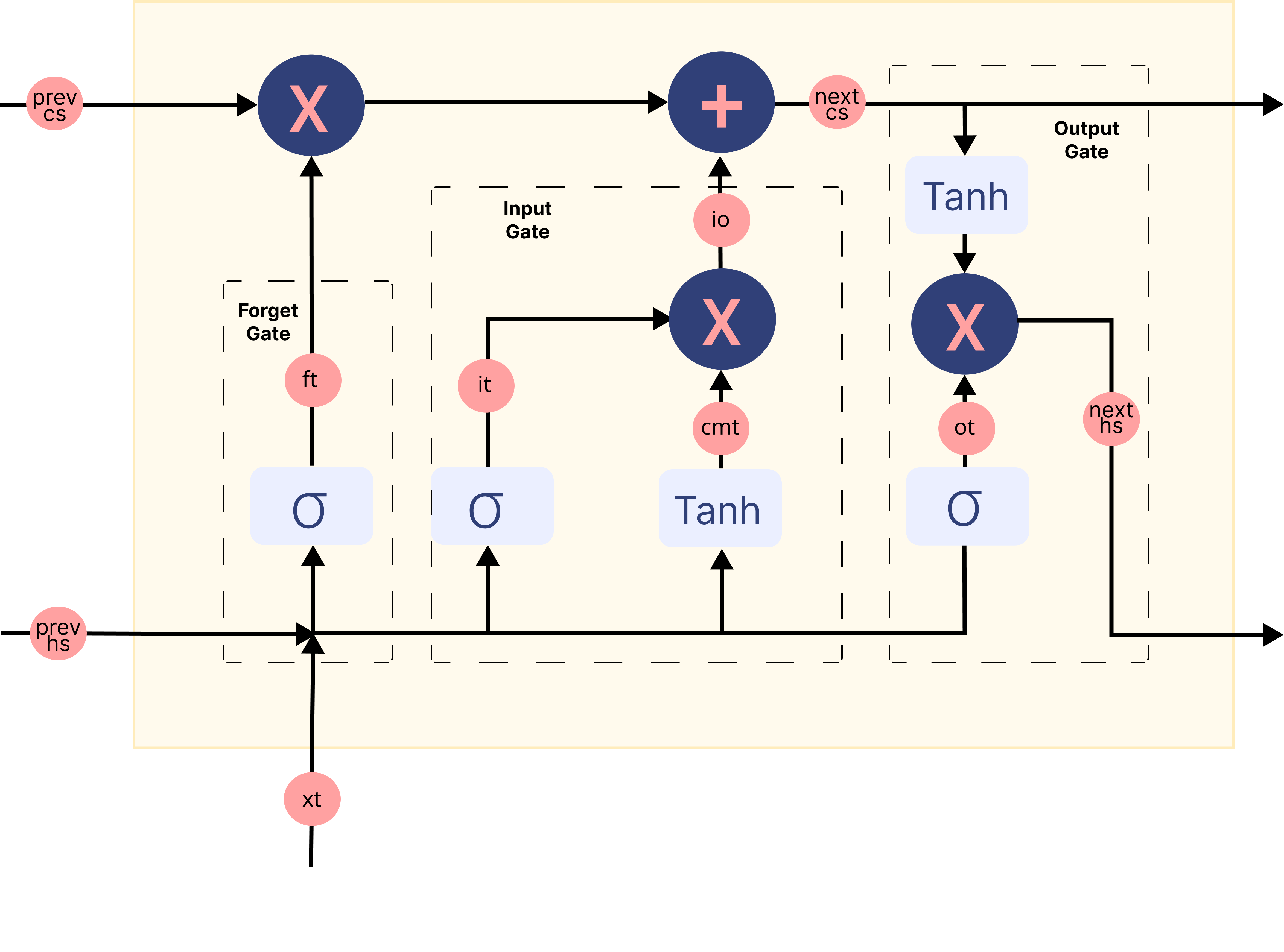
在上面的gif中,标记为 \(A\) 的矩形被称为 单元 ,它们是我们LSTM网络的 记忆块 。它们负责选择在序列中记住什么,并通过称为 隐藏状态 \(H_{t}\) 和 单元状态 \(C_{t}\) 的两个状态将该信息传递给下一个单元,其中 \(t\) 表示时间步。每个 单元 都有专门的门,负责存储、写入或读取传递给LSTM的信息。现在,您将通过实现其中发生的每个机制来仔细研究网络的架构。
让我们从编写一个函数开始,该函数将随机初始化在模型训练过程中学习的参数
def initialise_params(hidden_dim, input_dim):
    # forget gate
    Wf = rng.standard_normal(size=(hidden_dim, hidden_dim + input_dim))
    bf = rng.standard_normal(size=(hidden_dim, 1))
    # input gate
    Wi = rng.standard_normal(size=(hidden_dim, hidden_dim + input_dim))
    bi = rng.standard_normal(size=(hidden_dim, 1))
    # candidate memory gate
    Wcm = rng.standard_normal(size=(hidden_dim, hidden_dim + input_dim))
    bcm = rng.standard_normal(size=(hidden_dim, 1))
    # output gate
    Wo = rng.standard_normal(size=(hidden_dim, hidden_dim + input_dim))
    bo = rng.standard_normal(size=(hidden_dim, 1))

    # fully connected layer for classification
    W2 = rng.standard_normal(size=(1, hidden_dim))
    b2 = np.zeros((1, 1))

    parameters = {
        "Wf": Wf,
        "bf": bf,
        "Wi": Wi,
        "bi": bi,
        "Wcm": Wcm,
        "bcm": bcm,
        "Wo": Wo,
        "bo": bo,
        "W2": W2,
        "b2": b2
    }
    return parameters
前向传播#
既然你已经有了初始化的参数,你可以将输入数据通过网络正向传递。每一层接受输入数据,处理它并将它传递给下一层。这个过程被称为 前向传播 。你将采取以下机制来实现它:
加载输入数据的词嵌入
将嵌入传递给 LSTM
在LSTM的每个内存块中执行所有门机制,以获得最终的隐藏状态
通过全连接层传递最终隐藏状态以获得序列为正的概率
将所有计算的值存储在缓存中,以便在反向传播期间利用
Sigmoid 属于非线性激活函数家族。它帮助网络更新或遗忘数据。如果一个值的sigmoid结果为0,则认为信息被遗忘。同样,如果结果为1,信息保持不变。
def sigmoid(x):
    n = np.exp(np.fmin(x, 0))
    d = (1 + np.exp(-np.abs(x)))
    return n / d
遗忘门 将当前词嵌入和前一个隐藏状态连接在一起作为输入,并决定旧记忆单元内容中哪些部分需要关注,哪些可以忽略。
def fp_forget_gate(concat, parameters):
    ft = sigmoid(np.dot(parameters['Wf'], concat)
                 + parameters['bf'])
    return ft
输入门 将当前词嵌入和前一个隐藏状态连接在一起作为输入,并通过 候选记忆门 来控制我们通过 Tanh 函数调节流经网络的值,从而考虑多少新数据。
def fp_input_gate(concat, parameters):
    it = sigmoid(np.dot(parameters['Wi'], concat)
                 + parameters['bi'])
    cmt = np.tanh(np.dot(parameters['Wcm'], concat)
                  + parameters['bcm'])
    return it, cmt
最后我们有 输出门 ,它从当前词嵌入、前一个隐藏状态和已经通过遗忘门和输入门更新了信息的单元状态中获取信息,以更新隐藏状态的值。
def fp_output_gate(concat, next_cs, parameters):
    ot = sigmoid(np.dot(parameters['Wo'], concat)
                 + parameters['bo'])
    next_hs = ot * np.tanh(next_cs)
    return ot, next_hs
以下图像总结了LSTM网络内存块中的每个门机制:
图片已从 this 来源修改
但是你如何从LSTM的输出中获得情感?#
从序列中最后一个记忆块的输出门获得的隐藏状态被认为是序列中包含的所有信息的表示。为了将这些信息分类到不同的类别(在我们的例子中是2个,正面和负面),我们使用一个 全连接层 ,首先将这些信息映射到一个预定义的输出大小(在我们的例子中是1)。然后,一个激活函数(如sigmoid)将这个输出转换为0到1之间的值。我们认为大于0.5的值表示正面情绪。
def fp_fc_layer(last_hs, parameters):
    z2 = (np.dot(parameters['W2'], last_hs)
          + parameters['b2'])
    a2 = sigmoid(z2)
    return a2
现在,你将把这些函数结合起来,总结我们模型架构中的前向传播步骤:
def forward_prop(X_vec, parameters, input_dim):

    hidden_dim = parameters['Wf'].shape[0]
    time_steps = len(X_vec)

    # Initialise hidden and cell state before passing to first time step
    prev_hs = np.zeros((hidden_dim, 1))
    prev_cs = np.zeros(prev_hs.shape)

    # Store all the intermediate and final values here
    caches = {'lstm_values': [], 'fc_values': []}

    # Hidden state from the last cell in the LSTM layer is calculated.
    for t in range(time_steps):
        # Retrieve word corresponding to current time step
        x = X_vec[t]
        # Retrieve the embedding for the word and reshape it to make the LSTM happy
        xt = emb_matrix.get(x, rng.random(size=(input_dim, 1)))
        xt = xt.reshape((input_dim, 1))

        # Input to the gates is concatenated previous hidden state and current word embedding
        concat = np.vstack((prev_hs, xt))

        # Calculate output of the forget gate
        ft = fp_forget_gate(concat, parameters)

        # Calculate output of the input gate
        it, cmt = fp_input_gate(concat, parameters)
        io = it * cmt

        # Update the cell state
        next_cs = (ft * prev_cs) + io

        # Calculate output of the output gate
        ot, next_hs = fp_output_gate(concat, next_cs, parameters)

        # store all the values used and calculated by
        # the LSTM in a cache for backward propagation.
        lstm_cache = {
        "next_hs": next_hs,
        "next_cs": next_cs,
        "prev_hs": prev_hs,
        "prev_cs": prev_cs,
        "ft": ft,
        "it" : it,
        "cmt": cmt,
        "ot": ot,
        "xt": xt,
        }
        caches['lstm_values'].append(lstm_cache)

        # Pass the updated hidden state and cell state to the next time step
        prev_hs = next_hs
        prev_cs = next_cs

    # Pass the LSTM output through a fully connected layer to
    # obtain probability of the sequence being positive
    a2 = fp_fc_layer(next_hs, parameters)

    # store all the values used and calculated by the
    # fully connected layer in a cache for backward propagation.
    fc_cache = {
    "a2" : a2,
    "W2" : parameters['W2']
    }
    caches['fc_values'].append(fc_cache)
    return caches
反向传播#
在每次通过网络的前向传递之后,您将实现 通过时间的反向传播 算法,以在时间步长上累积每个参数的梯度。通过 LSTM 的反向传播不像通过其他常见的深度学习架构那样直接,因为其底层层的交互方式特殊。尽管如此,方法大体上是相同的;识别依赖关系并应用链式法则。
让我们从一个定义函数开始,该函数将每个参数的梯度初始化为由零组成的数组,其维度与相应参数相同
# Initialise the gradients
def initialize_grads(parameters):
    grads = {}
    for param in parameters.keys():
        grads[f'd{param}'] = np.zeros((parameters[param].shape))
    return grads
现在,对于每个门和全连接层,我们定义一个函数来计算损失相对于输入和使用参数的梯度。要理解导数计算背后的数学原理,我们建议您阅读Christina Kouridi的这篇有用的博客。
定义一个函数来计算 遗忘门 中的梯度:
def bp_forget_gate(hidden_dim, concat, dh_prev, dc_prev, cache, gradients, parameters):
    # dft = dL/da2 * da2/dZ2 * dZ2/dh_prev * dh_prev/dc_prev * dc_prev/dft
    dft = ((dc_prev * cache["prev_cs"] + cache["ot"]
           * (1 - np.square(np.tanh(cache["next_cs"])))
           * cache["prev_cs"] * dh_prev) * cache["ft"] * (1 - cache["ft"]))
    # dWf = dft * dft/dWf
    gradients['dWf'] += np.dot(dft, concat.T)
    # dbf = dft * dft/dbf
    gradients['dbf'] += np.sum(dft, axis=1, keepdims=True)
    # dh_f = dft * dft/dh_prev
    dh_f = np.dot(parameters["Wf"][:, :hidden_dim].T, dft)
    return dh_f, gradients
定义一个函数来计算 输入门 和 候选记忆门 中的梯度:
def bp_input_gate(hidden_dim, concat, dh_prev, dc_prev, cache, gradients, parameters):
    # dit = dL/da2 * da2/dZ2 * dZ2/dh_prev * dh_prev/dc_prev * dc_prev/dit
    dit = ((dc_prev * cache["cmt"] + cache["ot"]
           * (1 - np.square(np.tanh(cache["next_cs"])))
           * cache["cmt"] * dh_prev) * cache["it"] * (1 - cache["it"]))
    # dcmt = dL/da2 * da2/dZ2 * dZ2/dh_prev * dh_prev/dc_prev * dc_prev/dcmt
    dcmt = ((dc_prev * cache["it"] + cache["ot"]
            * (1 - np.square(np.tanh(cache["next_cs"])))
            * cache["it"] * dh_prev) * (1 - np.square(cache["cmt"])))
    # dWi = dit * dit/dWi
    gradients['dWi'] += np.dot(dit, concat.T)
    # dWcm = dcmt * dcmt/dWcm
    gradients['dWcm'] += np.dot(dcmt, concat.T)
    # dbi = dit * dit/dbi
    gradients['dbi'] += np.sum(dit, axis=1, keepdims=True)
    # dWcm = dcmt * dcmt/dbcm
    gradients['dbcm'] += np.sum(dcmt, axis=1, keepdims=True)
    # dhi = dit * dit/dh_prev
    dh_i = np.dot(parameters["Wi"][:, :hidden_dim].T, dit)
    # dhcm = dcmt * dcmt/dh_prev
    dh_cm = np.dot(parameters["Wcm"][:, :hidden_dim].T, dcmt)
    return dh_i, dh_cm, gradients
定义一个函数来计算 输出门 的梯度:
def bp_output_gate(hidden_dim, concat, dh_prev, dc_prev, cache, gradients, parameters):
    # dot = dL/da2 * da2/dZ2 * dZ2/dh_prev * dh_prev/dot
    dot = (dh_prev * np.tanh(cache["next_cs"])
           * cache["ot"] * (1 - cache["ot"]))
    # dWo = dot * dot/dWo
    gradients['dWo'] += np.dot(dot, concat.T)
    # dbo = dot * dot/dbo
    gradients['dbo'] += np.sum(dot, axis=1, keepdims=True)
    # dho = dot * dot/dho
    dh_o = np.dot(parameters["Wo"][:, :hidden_dim].T, dot)
    return dh_o, gradients
定义一个函数来计算 全连接层 的梯度:
def bp_fc_layer (target, caches, gradients):
    # dZ2 = dL/da2 * da2/dZ2
    predicted = np.array(caches['fc_values'][0]['a2'])
    target = np.array(target)
    dZ2 = predicted - target
    # dW2 = dL/da2 * da2/dZ2 * dZ2/dW2
    last_hs = caches['lstm_values'][-1]["next_hs"]
    gradients['dW2'] = np.dot(dZ2, last_hs.T)
    # db2 = dL/da2 * da2/dZ2 * dZ2/db2
    gradients['db2'] = np.sum(dZ2)
    # dh_last = dZ2 * W2
    W2 = caches['fc_values'][0]["W2"]
    dh_last = np.dot(W2.T, dZ2)
    return dh_last, gradients
将所有这些函数结合起来,总结我们模型的反向传播步骤:
def backprop(y, caches, hidden_dim, input_dim, time_steps, parameters):

    # Initialize gradients
    gradients = initialize_grads(parameters)

    # Calculate gradients for the fully connected layer
    dh_last, gradients = bp_fc_layer(target, caches, gradients)

    # Initialize gradients w.r.t previous hidden state and previous cell state
    dh_prev = dh_last
    dc_prev = np.zeros((dh_prev.shape))

    # loop back over the whole sequence
    for t in reversed(range(time_steps)):
        cache = caches['lstm_values'][t]

        # Input to the gates is concatenated previous hidden state and current word embedding
        concat = np.concatenate((cache["prev_hs"], cache["xt"]), axis=0)

        # Compute gates related derivatives
        # Calculate derivative w.r.t the input and parameters of forget gate
        dh_f, gradients = bp_forget_gate(hidden_dim, concat, dh_prev, dc_prev, cache, gradients, parameters)

        # Calculate derivative w.r.t the input and parameters of input gate
        dh_i, dh_cm, gradients = bp_input_gate(hidden_dim, concat, dh_prev, dc_prev, cache, gradients, parameters)

        # Calculate derivative w.r.t the input and parameters of output gate
        dh_o, gradients = bp_output_gate(hidden_dim, concat, dh_prev, dc_prev, cache, gradients, parameters)

        # Compute derivatives w.r.t prev. hidden state and the prev. cell state
        dh_prev = dh_f + dh_i + dh_cm + dh_o
        dc_prev = (dc_prev * cache["ft"] + cache["ot"]
                   * (1 - np.square(np.tanh(cache["next_cs"])))
                   * cache["ft"] * dh_prev)

    return gradients
更新参数#
我们通过一种称为 Adam 的优化算法来更新参数,这是对随机梯度下降的一种扩展,最近在计算机视觉和自然语言处理的深度学习应用中得到了更广泛的采用。具体来说,该算法计算梯度和平方梯度的指数移动平均值,参数 beta1 和 beta2 控制这些移动平均值的衰减率。Adam 相对于其他梯度下降算法显示出更高的收敛性和鲁棒性,通常被推荐为训练的默认优化器。
定义一个函数来初始化每个参数的移动平均值
# initialise the moving averages
def initialise_mav(hidden_dim, input_dim, params):
    v = {}
    s = {}
    # Initialize dictionaries v, s
    for key in params:
        v['d' + key] = np.zeros(params[key].shape)
        s['d' + key] = np.zeros(params[key].shape)
    # Return initialised moving averages
    return v, s
定义一个函数来更新参数
# Update the parameters using Adam optimization
def update_parameters(parameters, gradients, v, s,
                      learning_rate=0.01, beta1=0.9, beta2=0.999):
    for key in parameters:
        # Moving average of the gradients
        v['d' + key] = (beta1 * v['d' + key]
                        + (1 - beta1) * gradients['d' + key])

        # Moving average of the squared gradients
        s['d' + key] = (beta2 * s['d' + key]
                        + (1 - beta2) * (gradients['d' + key] ** 2))

        # Update parameters
        parameters[key] = (parameters[key] - learning_rate
                           * v['d' + key] / np.sqrt(s['d' + key] + 1e-8))
    # Return updated parameters and moving averages
    return parameters, v, s
训练网络#
首先,您将初始化网络中使用的所有参数和超参数
hidden_dim = 64
input_dim = emb_matrix['memory'].shape[0]
learning_rate = 0.001
epochs = 10
parameters = initialise_params(hidden_dim,
                               input_dim)
v, s = initialise_mav(hidden_dim,
                      input_dim,
                      parameters)
要优化你的深度学习网络,你需要根据模型在训练数据上的表现来计算损失。损失值表示每次优化迭代后模型的表现好坏。
定义一个函数,使用 负对数似然 来计算损失。
def loss_f(A, Y):
    # define value of epsilon to prevent zero division error inside a log
    epsilon = 1e-5
    # Implement formula for negative log likelihood
    loss = (- Y * np.log(A + epsilon)
            - (1 - Y) * np.log(1 - A + epsilon))
    # Return loss
    return np.squeeze(loss)
设置神经网络的学习实验,使用训练循环并开始训练过程。您还将评估模型在训练数据集上的表现,以查看模型的学习效果,以及在测试数据集上的表现,以查看模型的泛化效果。
如果已经在
npy文件中存储了训练好的参数,则跳过运行此单元格
# To store training losses
training_losses = []
# To store testing losses
testing_losses = []

# This is a training loop.
# Run the learning experiment for a defined number of epochs (iterations).
for epoch in range(epochs):
    #################
    # Training step #
    #################
    train_j = []
    for sample, target in zip(X_train, y_train):
        # split text sample into words/tokens
        b = textproc.word_tokeniser(sample)

        # Forward propagation/forward pass:
        caches = forward_prop(b,
                              parameters,
                              input_dim)

        # Backward propagation/backward pass:
        gradients = backprop(target,
                             caches,
                             hidden_dim,
                             input_dim,
                             len(b),
                             parameters)

        # Update the weights and biases for the LSTM and fully connected layer
        parameters, v, s = update_parameters(parameters,
                                             gradients,
                                             v,
                                             s,
                                             learning_rate=learning_rate,
                                             beta1=0.999,
                                             beta2=0.9)

        # Measure the training error (loss function) between the actual
        # sentiment (the truth) and the prediction by the model.
        y_pred = caches['fc_values'][0]['a2'][0][0]
        loss = loss_f(y_pred, target)
        # Store training set losses
        train_j.append(loss)

    ###################
    # Evaluation step #
    ###################
    test_j = []
    for sample, target in zip(X_test, y_test):
        # split text sample into words/tokens
        b = textproc.word_tokeniser(sample)

        # Forward propagation/forward pass:
        caches = forward_prop(b,
                              parameters,
                              input_dim)

        # Measure the testing error (loss function) between the actual
        # sentiment (the truth) and the prediction by the model.
        y_pred = caches['fc_values'][0]['a2'][0][0]
        loss = loss_f(y_pred, target)

        # Store testing set losses
        test_j.append(loss)

    # Calculate average of training and testing losses for one epoch
    mean_train_cost = np.mean(train_j)
    mean_test_cost = np.mean(test_j)
    training_losses.append(mean_train_cost)
    testing_losses.append(mean_test_cost)
    print('Epoch {} finished. \t  Training Loss : {} \t  Testing Loss : {}'.
          format(epoch + 1, mean_train_cost, mean_test_cost))

# save the trained parameters to a npy file
np.save('tutorial-nlp-from-scratch/parameters.npy', parameters)
绘制训练和测试损失作为学习曲线通常有助于诊断机器学习模型的行为,这是一个很好的做法。
fig = plt.figure()
ax = fig.add_subplot(111)

# plot the training loss
ax.plot(range(0, len(training_losses)), training_losses, label='training loss')
# plot the testing loss
ax.plot(range(0, len(testing_losses)), testing_losses, label='testing loss')

# set the x and y labels
ax.set_xlabel("epochs")
ax.set_ylabel("loss")

plt.legend(title='labels', bbox_to_anchor=(1.0, 1), loc='upper left')
plt.show()
演讲数据的情感分析#
一旦你的模型训练完成,你可以使用更新后的参数开始进行预测。你可以在将每段演讲分解成统一大小的段落后再传递给深度学习模型,并预测每个段落的情感。
# To store predicted sentiments
predictions = {}

# define the length of a paragraph
para_len = 100

# Retrieve trained values of the parameters
if os.path.isfile('tutorial-nlp-from-scratch/parameters.npy'):
    parameters = np.load('tutorial-nlp-from-scratch/parameters.npy', allow_pickle=True).item()

# This is the prediction loop.
for index, text in enumerate(X_pred):
    # split each speech into paragraphs
    paras = textproc.text_to_paras(text, para_len)
    # To store the network outputs
    preds = []

    for para in paras:
        # split text sample into words/tokens
        para_tokens = textproc.word_tokeniser(para)
        # Forward Propagation
        caches = forward_prop(para_tokens,
                              parameters,
                              input_dim)

        # Retrieve the output of the fully connected layer
        sent_prob = caches['fc_values'][0]['a2'][0][0]
        preds.append(sent_prob)

    threshold = 0.5
    preds = np.array(preds)
    # Mark all predictions > threshold as positive and < threshold as negative
    pos_indices = np.where(preds > threshold)  # indices where output > 0.5
    neg_indices = np.where(preds < threshold)  # indices where output < 0.5
    # Store predictions and corresponding piece of text
    predictions[speakers[index]] = {'pos_paras': paras[pos_indices[0]],
                                    'neg_paras': paras[neg_indices[0]]}
可视化情感预测:
x_axis = []
data = {'positive sentiment': [], 'negative sentiment': []}
for speaker in predictions:
    # The speakers will be used to label the x-axis in our plot
    x_axis.append(speaker)
    # number of paras with positive sentiment
    no_pos_paras = len(predictions[speaker]['pos_paras'])
    # number of paras with negative sentiment
    no_neg_paras = len(predictions[speaker]['neg_paras'])
    # Obtain percentage of paragraphs with positive predicted sentiment
    pos_perc = no_pos_paras / (no_pos_paras + no_neg_paras)
    # Store positive and negative percentages
    data['positive sentiment'].append(pos_perc*100)
    data['negative sentiment'].append(100*(1-pos_perc))

index = pd.Index(x_axis, name='speaker')
df = pd.DataFrame(data, index=index)
ax = df.plot(kind='bar', stacked=True)
ax.set_ylabel('percentage')
ax.legend(title='labels', bbox_to_anchor=(1, 1), loc='upper left')
plt.show()
在上面的图中,您可以看到每段话中预期带有正面和负面情绪的百分比。由于这个实现优先考虑简单性和清晰性而非性能,我们不能期望这些结果非常准确。此外,在为一个段落做情绪预测时,我们没有使用相邻段落作为上下文,这本可以导致更准确的预测。我们鼓励读者尝试使用该模型,并根据 下一步 中的建议进行一些调整,观察模型性能的变化。
从伦理角度看我们的神经网络#
准确识别文本的情感并不容易,这主要是因为人类表达情感的方式复杂,使用讽刺、 sarcasm、幽默或社交媒体中的缩写。此外,将文本整齐地分为‘正面’和‘负面’两类可能会有问题,因为这样做时没有考虑任何上下文。词语或缩写可以根据年龄和地点传达非常不同的情感,这些我们在构建模型时都没有考虑到。
除了数据之外,人们也越来越担心数据处理算法正在以不透明的方式影响政策和日常生活,并引入了偏见。某些偏见,例如 归纳偏见 对于帮助机器学习模型更好地泛化是必要的,例如我们之前构建的 LSTM 偏向于在长序列中保留上下文信息,这使得它非常适合处理序列数据。问题出现在 社会偏见 潜入算法预测中。通过 超参数调优 等方法优化机器算法,可能会通过学习数据中的每一点信息进一步放大这些偏见。
也存在偏见仅出现在输出而非输入(数据、算法)的情况。例如,在情感分析中 女性撰写的文本的准确性往往高于男性撰写的文本。情感分析的终端用户应意识到其微小的性别偏见可能会影响从中得出的结论,并在必要时应用修正因子。因此,重要的是,对算法责任的要求应包括测试系统输出的能力,包括按性别、种族和其他特征深入不同用户组的能力,以识别并希望提出系统输出偏见的修正。
下一步#
你已经学会了如何使用仅 NumPy 从头构建和训练一个简单的长短期记忆网络,以执行情感分析。
为了进一步增强和优化你的神经网络模型,你可以考虑以下混合方法之一:
通过引入多个 LSTM 层来改变架构,使网络更深。
使用更高的 epoch 大小来训练更长时间,并添加更多的正则化技术,例如早停,以防止过拟合。
引入一个验证集以对模型拟合进行无偏评估。
应用批量归一化以实现更快和更稳定的训练。
调整其他参数,例如学习率和隐藏层大小。
使用 Xavier Initialization 初始化权重以防止梯度消失/爆炸,而不是随机初始化它们。
将 LSTM 替换为 双向 LSTM 以使用左右上下文来预测情感。
如今,LSTM 已经被 Transformer 取代(它使用 Attention 来解决困扰 LSTM 的所有问题,例如缺乏 迁移学习、缺乏 并行训练 以及长序列的长梯度链)
使用 NumPy 从头构建一个神经网络是学习更多关于 NumPy 和深度学习的一个好方法。然而,对于实际应用,你应该使用专门的框架——例如 PyTorch、JAX 或 TensorFlow——它们提供类似 NumPy 的 API,内置自动微分和 GPU 支持,并且设计用于高性能数值计算和机器学习。
最后,要了解更多关于在开发机器学习模型时伦理如何发挥作用的信息,您可以参考以下资源:
图灵研究所的数据伦理资源。 https://www.turing.ac.uk/research/data-ethics
更多伦理资源请参见 Rachel Thomas 的 这篇博客文章 和 Radical AI 播客