如何使用自定义数据并实现自定义模型和指标#
在PyTorch Forecasting中构建新模型相对容易。许多事情都是自动处理的
对于大多数模型,训练、验证和推理是自动处理的 - 定义架构和超参数就足够了
数据加载、归一化、重新缩放等由TimeSeriesDataSet提供
自动处理包括绘制示例在内的多个指标的训练进度记录
如果不同的时间序列具有不同的长度,条目的掩码是自动的
然而,如果你想充分利用这个包,有几件事情需要记住。本教程首先演示如何实现一个简单的模型,然后转向更复杂的实现场景。
我们将回答以下问题
如何将现有的PyTorch实现转换为PyTorch Forecasting
如何处理数据加载并启用不同长度的时间序列
如何定义和使用自定义指标
如何处理循环网络
如何处理协变量
如何测试新模型
构建一个简单的初始模型#
为了演示目的,我们将选择一个简单的全连接模型。它接受大小为input_size的时间序列作为输入,并输出大小为output_size的新时间序列。你可以将这个input_size视为编码步骤,将output_size视为解码/预测步骤。
[1]:
import warnings

warnings.filterwarnings("ignore")
[2]:
import torch
from torch import nn


class FullyConnectedModule(nn.Module):
    def __init__(self, input_size: int, output_size: int, hidden_size: int, n_hidden_layers: int):
        super().__init__()

        # input layer
        module_list = [nn.Linear(input_size, hidden_size), nn.ReLU()]
        # hidden layers
        for _ in range(n_hidden_layers):
            module_list.extend([nn.Linear(hidden_size, hidden_size), nn.ReLU()])
        # output layer
        module_list.append(nn.Linear(hidden_size, output_size))

        self.sequential = nn.Sequential(*module_list)

    def forward(self, x: torch.Tensor) -> torch.Tensor:
        # x of shape: batch_size x n_timesteps_in
        # output of shape batch_size x n_timesteps_out
        return self.sequential(x)


# test that network works as intended
network = FullyConnectedModule(input_size=5, output_size=2, hidden_size=10, n_hidden_layers=2)
x = torch.rand(20, 5)
network(x).shape
[2]:
torch.Size([20, 2])
上述模型还不是一个PyTorch Forecasting模型,但很容易实现。由于这是一个简单的模型,我们将使用BaseModel。这个基类是修改后的LightningModule,具有预定义的钩子用于训练和验证时间序列模型。BaseModelWithCovariates将在本教程的后面讨论。
无论哪种方式,主要要求是模型要有一个forward方法。
- BaseModel.forward(x: Dict[str, List[Tensor] | Tensor]) Dict[str, List[Tensor] | Tensor][来源]
网络前向传播。
- Parameters:
x (Dict[str, Union[torch.Tensor, List[torch.Tensor]]]) – 网络输入(x 由数据加载器返回)。 参见
to_dataloader()方法, 该方法返回一个包含x和y的元组。此函数期望x。- Returns:
- 网络输出 / 张量字典或列表
使用
to_network_output()方法创建它。 字典中所需的最小条目是(以及括号中的形状):prediction(batch_size x n_decoder_time_steps x n_outputs 或每个条目对应不同目标的列表):可以输入到度量中的重新缩放的预测。如果同时预测多个目标,则为张量列表。
在输出预测之前,您需要将它们重新缩放到实际空间。 默认情况下,您可以使用
transform_output()方法来实现这一点。
- Return type:
NamedTuple[Union[torch.Tensor, List[torch.Tensor]]
示例
def forward(self, x:
    # x is a batch generated based on the TimeSeriesDataset, here we just use the
    # continuous variables for the encoder
    network_input = x["encoder_cont"].squeeze(-1)
    prediction = self.linear(network_input)  #

    # rescale predictions into target space
    prediction = self.transform_output(prediction, target_scale=x["target_scale"])

    # We need to return a dictionary that at least contains the prediction
    # The parameter can be directly forwarded from the input.
    # The conversion to a named tuple can be directly achieved with the `to_network_output` function.
    return self.to_network_output(prediction=prediction)
[3]:
from typing import Dict

from pytorch_forecasting.models import BaseModel


class FullyConnectedModel(BaseModel):
    def __init__(self, input_size: int, output_size: int, hidden_size: int, n_hidden_layers: int, **kwargs):
        # saves arguments in signature to `.hparams` attribute, mandatory call - do not skip this
        self.save_hyperparameters()
        # pass additional arguments to BaseModel.__init__, mandatory call - do not skip this
        super().__init__(**kwargs)
        self.network = FullyConnectedModule(
            input_size=self.hparams.input_size,
            output_size=self.hparams.output_size,
            hidden_size=self.hparams.hidden_size,
            n_hidden_layers=self.hparams.n_hidden_layers,
        )

    def forward(self, x: Dict[str, torch.Tensor]) -> Dict[str, torch.Tensor]:
        # x is a batch generated based on the TimeSeriesDataset
        network_input = x["encoder_cont"].squeeze(-1)
        prediction = self.network(network_input)

        # rescale predictions into target space
        prediction = self.transform_output(prediction, target_scale=x["target_scale"])

        # We need to return a dictionary that at least contains the prediction
        # The parameter can be directly forwarded from the input.
        # The conversion to a named tuple can be directly achieved with the `to_network_output` function.
        return self.to_network_output(prediction=prediction)
这是一个非常基础的实现,可以立即用于训练。但在我们添加额外功能之前,让我们先看看在初始化模型之前如何将数据传递给这个模型。
将数据传递给模型#
我们可以利用 PyTorch Forecasting 的 TimeSeriesDataSet 来为我们的模型提供数据,而不必编写自己的数据加载器(这可能相当复杂)。
事实上,PyTorch Forecasting 希望我们使用 TimeSeriesDataSet。
数据必须采用特定格式才能被TimeSeriesDataSet使用。它应该是一个pandas DataFrame,并且有一个分类列来标识每个系列,以及一个整数列来指定记录的时间。
下面,我们创建了一个包含30个不同观测值的数据集 - 每个时间序列有10个观测值。
[4]:
import numpy as np
import pandas as pd

test_data = pd.DataFrame(
    dict(
        value=np.random.rand(30) - 0.5,
        group=np.repeat(np.arange(3), 10),
        time_idx=np.tile(np.arange(10), 3),
    )
)
test_data
[4]:
| 值 | 组 | 时间索引 | |
|---|---|---|---|
| 0 | -0.125597 | 0 | 0 |
| 1 | 0.325668 | 0 | 1 |
| 2 | -0.265962 | 0 | 2 |
| 3 | 0.132305 | 0 | 3 |
| 4 | 0.167117 | 0 | 4 |
| 5 | 0.481241 | 0 | 5 |
| 6 | -0.113188 | 0 | 6 |
| 7 | -0.089609 | 0 | 7 |
| 8 | 0.029156 | 0 | 8 |
| 9 | -0.181950 | 0 | 9 |
| 10 | 0.150334 | 1 | 0 |
| 11 | 0.428624 | 1 | 1 |
| 12 | -0.139106 | 1 | 2 |
| 13 | -0.085334 | 1 | 3 |
| 14 | -0.243668 | 1 | 4 |
| 15 | 0.055913 | 1 | 5 |
| 16 | 0.308591 | 1 | 6 |
| 17 | 0.141183 | 1 | 7 |
| 18 | 0.230759 | 1 | 8 |
| 19 | 0.173528 | 1 | 9 |
| 20 | 0.226315 | 2 | 0 |
| 21 | -0.348390 | 2 | 1 |
| 22 | 0.067816 | 2 | 2 |
| 23 | -0.074794 | 2 | 3 |
| 24 | 0.059396 | 2 | 4 |
| 25 | 0.300745 | 2 | 5 |
| 26 | -0.344032 | 2 | 6 |
| 27 | -0.083934 | 2 | 7 |
| 29 | -0.385202 | 2 | 9 |
将其转换为TimeSeriesDataSet非常简单:
[5]:
from pytorch_forecasting import TimeSeriesDataSet

# create the dataset from the pandas dataframe
dataset = TimeSeriesDataSet(
    test_data,
    group_ids=["group"],
    target="value",
    time_idx="time_idx",
    min_encoder_length=5,
    max_encoder_length=5,
    min_prediction_length=2,
    max_prediction_length=2,
    time_varying_unknown_reals=["value"],
)
我们可以查看由PyTorch Forecasting设置的所有默认值和设置。这些都可以作为TimeSeriesDataSet的参数使用 - 有关所有详细信息,请参阅其文档。
[6]:
dataset.get_parameters()
[6]:
{'time_idx': 'time_idx',
 'target': 'value',
 'group_ids': ['group'],
 'weight': None,
 'max_encoder_length': 5,
 'min_encoder_length': 5,
 'min_prediction_idx': 0,
 'min_prediction_length': 2,
 'max_prediction_length': 2,
 'static_categoricals': [],
 'static_reals': [],
 'time_varying_known_categoricals': [],
 'time_varying_known_reals': [],
 'time_varying_unknown_categoricals': [],
 'time_varying_unknown_reals': ['value'],
 'variable_groups': {},
 'constant_fill_strategy': {},
 'allow_missing_timesteps': False,
 'lags': {},
 'add_relative_time_idx': False,
 'add_target_scales': False,
 'add_encoder_length': False,
 'target_normalizer': GroupNormalizer(
        method='standard',
        groups=[],
        center=True,
        scale_by_group=False,
        transformation=None,
        method_kwargs={}
 ),
 'categorical_encoders': {'__group_id__group': NaNLabelEncoder(add_nan=False, warn=True),
  'group': NaNLabelEncoder(add_nan=False, warn=True)},
 'scalers': {},
 'randomize_length': None,
 'predict_mode': False}
现在,我们来看一下数据加载器的输出。它的x将被输入到模型的前向方法中,这就是为什么理解它如此重要。
[7]:
# convert the dataset to a dataloader
dataloader = dataset.to_dataloader(batch_size=4)

# and load the first batch
x, y = next(iter(dataloader))
print("x =", x)
print("\ny =", y)
print("\nsizes of x =")
for key, value in x.items():
    print(f"\t{key} = {value.size()}")
x = {'encoder_cat': tensor([], size=(4, 5, 0), dtype=torch.int64), 'encoder_cont': tensor([[[ 1.7401],
         [-0.6492],
         [-0.4229],
         [-1.0892],
         [ 0.1716]],

        [[-0.4229],
         [-1.0892],
         [ 0.1716],
         [ 1.2349],
         [ 0.5304]],

        [[-0.6492],
         [-0.4229],
         [-1.0892],
         [ 0.1716],
         [ 1.2349]],

        [[-1.5299],
         [ 0.2216],
         [-0.3785],
         [ 0.1862],
         [ 1.2019]]]), 'encoder_target': tensor([[ 0.4286, -0.1391, -0.0853, -0.2437,  0.0559],
        [-0.0853, -0.2437,  0.0559,  0.3086,  0.1412],
        [-0.1391, -0.0853, -0.2437,  0.0559,  0.3086],
        [-0.3484,  0.0678, -0.0748,  0.0594,  0.3007]]), 'encoder_lengths': tensor([5, 5, 5, 5]), 'decoder_cat': tensor([], size=(4, 2, 0), dtype=torch.int64), 'decoder_cont': tensor([[[ 1.2349],
         [ 0.5304]],

        [[ 0.9074],
         [ 0.6665]],

        [[ 0.5304],
         [ 0.9074]],

        [[-1.5116],
         [-0.4170]]]), 'decoder_target': tensor([[ 0.3086,  0.1412],
        [ 0.2308,  0.1735],
        [ 0.1412,  0.2308],
        [-0.3440, -0.0839]]), 'decoder_lengths': tensor([2, 2, 2, 2]), 'decoder_time_idx': tensor([[6, 7],
        [8, 9],
        [7, 8],
        [6, 7]]), 'groups': tensor([[1],
        [1],
        [1],
        [2]]), 'target_scale': tensor([[0.0151, 0.2376],
        [0.0151, 0.2376],
        [0.0151, 0.2376],
        [0.0151, 0.2376]])}

y = (tensor([[ 0.3086,  0.1412],
        [ 0.2308,  0.1735],
        [ 0.1412,  0.2308],
        [-0.3440, -0.0839]]), None)

sizes of x =
        encoder_cat = torch.Size([4, 5, 0])
        encoder_cont = torch.Size([4, 5, 1])
        encoder_target = torch.Size([4, 5])
        encoder_lengths = torch.Size([4])
        decoder_cat = torch.Size([4, 2, 0])
        decoder_cont = torch.Size([4, 2, 1])
        decoder_target = torch.Size([4, 2])
        decoder_lengths = torch.Size([4])
        decoder_time_idx = torch.Size([4, 2])
        groups = torch.Size([4, 1])
        target_scale = torch.Size([4, 2])
为了更好地理解它,我们查看to_dataloader()方法的文档:
- TimeSeriesDataSet.to_dataloader(train: bool = True, batch_size: int = 64, batch_sampler: Sampler | str = None, **kwargs) DataLoader[来源]
从数据集构建数据加载器,用于模型。
- Parameters:
train (bool, optional, default=Trze) – 数据加载器是否用于训练(True)或预测(False)。 如果为True,将打乱数据并丢弃最后一批。默认为True。
batch_size (int, optional, default=64) – 训练模型的批量大小。默认为64。
batch_sampler (Sampler, str, or None, optional, default=None) –
torch 批量采样器或字符串。其中之一
- ”synchronized”: 确保解码器中的样本在时间上对齐。
不支持数据集中的缺失值。 这只有在底层算法使用时间对齐的值时才有意义。
- PyTorch 采样器实例: 任何 PyTorch 采样器,
例如,
the WeightedRandomSampler()
None: 样本从时间序列中随机抽取。
**kwargs(传递给
DataLoader构造函数的额外参数)
- Returns:
DataLoader – 第一个条目是
x,一个包含条目和张量形状的字典。- encoder_catlong (batch_size x n_encoder_time_steps x n_features)
编码器的长张量,包含编码的分类数据
- encoder_contfloat (batch_size x n_encoder_time_steps x n_features)
编码器的浮点张量,包含缩放的连续变量
- encoder_targetfloat (batch_size x n_encoder_time_steps) 或其列表
如果是列表,每个条目对应不同的目标。 未缩放的连续目标或编码的分类目标的浮点张量, 多个目标的张量列表
- encoder_lengthslong (batch_size)
编码器时间序列长度的长张量。没有条目会超过 n_encoder_time_steps
- decoder_catlong (batch_size x n_decoder_time_steps x n_features)
解码器的长张量,包含编码的分类数据
- decoder_contfloat (batch_size x n_decoder_time_steps x n_features)
解码器的浮点张量,包含缩放的连续变量
- decoder_targetfloat (batch_size x n_decoder_time_steps) 或其列表
如果是列表,每个条目对应不同的目标。 未缩放的连续目标或编码的分类目标的浮点张量, 多个目标的张量列表
- decoder_lengthslong (batch_size)
解码器时间序列长度的长张量。没有条目会超过 n_decoder_time_steps
- group_idsfloat (batch_size x number_of_ids)
标识数据集中时间序列的编码组ID
- target_scalefloat (batch_size x scale_size) 或其列表
如果是列表,每个条目对应不同的目标。 用于归一化目标的参数。 通常是均值和标准差。 多个目标的张量列表。
第二个条目是
y,一个形式为 (target, weight) 的元组- targetfloat (batch_size x n_decoder_time_steps) 或其列表
如果是列表,每个条目对应不同的目标。 未缩放(连续)或编码(分类)的目标, 多个目标的张量列表
- weightNone 或 float (batch_size x n_decoder_time_steps)
每个目标的权重,如果未使用权重则为 None(= 等权重)
- Return type:
返回元组的数据加载器。
示例
训练样本的权重:
from torch.utils.data import WeightedRandomSampler

# length of probabilties for sampler have to be equal to the length of index
probabilities = np.sqrt(1 + data.loc[dataset.index, "target"])
sampler = WeightedRandomSampler(probabilities, len(probabilities))
dataset.to_dataloader(train=True, sampler=sampler, shuffle=False)
这解释了为什么在我们上面的简单FullyConnectedModel中,我们必须首先提取正确的输入,然后再将其传递给我们的FullyConnectedModule。提醒一下:
[8]:
def forward(self, x: Dict[str, torch.Tensor]) -> Dict[str, torch.Tensor]:
    # x is a batch generated based on the TimeSeriesDataset
    network_input = x["encoder_cont"].squeeze(-1)
    prediction = self.network(network_input)

    # rescale predictions into target space
    prediction = self.transform_output(prediction, target_scale=x["target_scale"])

    # We need to return a dictionary that at least contains the prediction
    # The parameter can be directly forwarded from the input.
    # The conversion to a named tuple can be directly achieved with the `to_network_output` function.
    return self.to_network_output(prediction=prediction)
对于这样一个简单的架构,我们可以忽略x中的大部分输入。您不必担心将张量移动到特定的GPU,PyTorch Lightning会为您处理这个问题。
现在,让我们检查一下我们的模型是否有效。我们总是使用他们的from_dataset()方法来初始化模型,该方法从数据集中获取超参数、模型的超参数和优化器的超参数。在下一节中了解更多信息。
[9]:
model = FullyConnectedModel.from_dataset(dataset, input_size=5, output_size=2, hidden_size=10, n_hidden_layers=2)
x, y = next(iter(dataloader))
model(x)
[9]:
Output(prediction=tensor([[-0.0175, -0.0045],
        [-0.0203,  0.0039],
        [-0.0128,  0.0033],
        [-0.0162, -0.0026]], grad_fn=<AddBackward0>))
如果你想知道批次中的样本链接到哪个组和时间索引(在第一次预测时),你可以通过使用x_to_index()来找出:
[10]:
dataset.x_to_index(x)
[10]:
| 时间索引 | 组别 | |
|---|---|---|
| 0 | 5 | 2 |
| 1 | 5 | 1 |
| 2 | 7 | 2 |
| 3 | 5 | 0 |
耦合数据集和模型#
你可能已经注意到,编码器和解码器/预测长度(5和2)已经在TimeSeriesDataSet中指定,并且我们在初始化模型时再次指定了它们。对于这样一个简单的模型来说,这可能是可以接受的,但在更复杂的情况下,这将使用户难以理解如何从数据集映射到模型参数。
这就是为什么我们应该在模型中实现另一个方法:from_dataset()。通常,用户总是会从数据集初始化模型。该方法也是一个验证用户定义的数据集是否与你的模型架构兼容的机会。
虽然TimeSeriesDataSet和所有PyTorch Forecasting指标支持不同长度的时间序列,但并非每个网络架构都支持。
[11]:
class FullyConnectedModel(BaseModel):
    def __init__(self, input_size: int, output_size: int, hidden_size: int, n_hidden_layers: int, **kwargs):
        # saves arguments in signature to `.hparams` attribute, mandatory call - do not skip this
        self.save_hyperparameters()
        # pass additional arguments to BaseModel.__init__, mandatory call - do not skip this
        super().__init__(**kwargs)
        self.network = FullyConnectedModule(
            input_size=self.hparams.input_size,
            output_size=self.hparams.output_size,
            hidden_size=self.hparams.hidden_size,
            n_hidden_layers=self.hparams.n_hidden_layers,
        )

    def forward(self, x: Dict[str, torch.Tensor]) -> Dict[str, torch.Tensor]:
        # x is a batch generated based on the TimeSeriesDataset
        network_input = x["encoder_cont"].squeeze(-1)
        prediction = self.network(network_input).unsqueeze(-1)

        # rescale predictions into target space
        prediction = self.transform_output(prediction, target_scale=x["target_scale"])

        # We need to return a dictionary that at least contains the prediction.
        # The parameter can be directly forwarded from the input.
        # The conversion to a named tuple can be directly achieved with the `to_network_output` function.
        return self.to_network_output(prediction=prediction)

    @classmethod
    def from_dataset(cls, dataset: TimeSeriesDataSet, **kwargs):
        new_kwargs = {
            "output_size": dataset.max_prediction_length,
            "input_size": dataset.max_encoder_length,
        }
        new_kwargs.update(kwargs)  # use to pass real hyperparameters and override defaults set by dataset
        # example for dataset validation
        assert dataset.max_prediction_length == dataset.min_prediction_length, "Decoder only supports a fixed length"
        assert dataset.min_encoder_length == dataset.max_encoder_length, "Encoder only supports a fixed length"
        assert (
            len(dataset._time_varying_known_categoricals) == 0
            and len(dataset._time_varying_known_reals) == 0
            and len(dataset._time_varying_unknown_categoricals) == 0
            and len(dataset._static_categoricals) == 0
            and len(dataset._static_reals) == 0
            and len(dataset._time_varying_unknown_reals) == 1
            and dataset._time_varying_unknown_reals[0] == dataset.target
        ), "Only covariate should be the target in 'time_varying_unknown_reals'"

        return super().from_dataset(dataset, **new_kwargs)
现在,让我们从我们的数据集中初始化:
[12]:
from lightning.pytorch.utilities.model_summary import ModelSummary

model = FullyConnectedModel.from_dataset(dataset, hidden_size=10, n_hidden_layers=2)
print(ModelSummary(model, max_depth=-1))
model.hparams
   | Name                 | Type                 | Params
---------------------------------------------------------------
0  | loss                 | SMAPE                | 0
1  | logging_metrics      | ModuleList           | 0
2  | network              | FullyConnectedModule | 302
3  | network.sequential   | Sequential           | 302
4  | network.sequential.0 | Linear               | 60
5  | network.sequential.1 | ReLU                 | 0
6  | network.sequential.2 | Linear               | 110
7  | network.sequential.3 | ReLU                 | 0
8  | network.sequential.4 | Linear               | 110
9  | network.sequential.5 | ReLU                 | 0
10 | network.sequential.6 | Linear               | 22
---------------------------------------------------------------
302       Trainable params
0         Non-trainable params
302       Total params
0.001     Total estimated model params size (MB)
[12]:
"hidden_size":                 10
"input_size":                  5
"learning_rate":               0.001
"log_gradient_flow":           False
"log_interval":                -1
"log_val_interval":            -1
"logging_metrics":             ModuleList()
"loss":                        SMAPE()
"monotone_constaints":         {}
"n_hidden_layers":             2
"optimizer":                   ranger
"optimizer_params":            None
"output_size":                 2
"output_transformer":          GroupNormalizer(
        method='standard',
        groups=[],
        center=True,
        scale_by_group=False,
        transformation=None,
        method_kwargs={}
)
"reduce_on_plateau_min_lr":    1e-05
"reduce_on_plateau_patience":  1000
"reduce_on_plateau_reduction": 2.0
"weight_decay":                0.0
定义额外的超参数#
到目前为止,我们在模型初始化签名中保留了一个通配符 **kwargs 参数。然后我们通过 super().__init__(**kwargs) 调用将这些 **kwargs 传递给 BaseModel。我们可以看到哪些额外的超参数是可用的,因为它们都保存在模型的 hparams 属性中:
[13]:
model.hparams
[13]:
"hidden_size":                 10
"input_size":                  5
"learning_rate":               0.001
"log_gradient_flow":           False
"log_interval":                -1
"log_val_interval":            -1
"logging_metrics":             ModuleList()
"loss":                        SMAPE()
"monotone_constaints":         {}
"n_hidden_layers":             2
"optimizer":                   ranger
"optimizer_params":            None
"output_size":                 2
"output_transformer":          GroupNormalizer(
        method='standard',
        groups=[],
        center=True,
        scale_by_group=False,
        transformation=None,
        method_kwargs={}
)
"reduce_on_plateau_min_lr":    1e-05
"reduce_on_plateau_patience":  1000
"reduce_on_plateau_reduction": 2.0
"weight_decay":                0.0
虽然不是必需的,但为了让用户对这些额外的超参数有透明度,值得明确地传递它们,而不是隐式地在**kwargs中传递。
它们在BaseModel中有详细描述。
- BaseModel.__init__(dataset_parameters: Dict[str, Any] = None, log_interval: int | float = -1, log_val_interval: int | float = None, learning_rate: float | List[float] = 0.001, log_gradient_flow: bool = False, loss: 指标 = SMAPE(), logging_metrics: ModuleList = ModuleList(), reduce_on_plateau_patience: int = 1000, reduce_on_plateau_reduction: float = 2.0, reduce_on_plateau_min_lr: float = 1e-05, weight_decay: float = 0.0, optimizer_params: Dict[str, Any] = None, monotone_constraints: Dict[str, int] = {}, output_transformer: Callable = None, optimizer='adam')[来源]
用于时间序列预测的BaseModel,可以从中继承
- Parameters:
log_interval (Union[int, float], optional) – 在此批次之后记录预测结果。如果小于1.0,则每批次将记录多个条目。默认为-1。
log_val_interval (Union[int, float], optional) – 在多少个批次后记录验证的预测结果。默认为 None/log_interval。
learning_rate (float, optional) – 学习率。默认为 1e-3。
log_gradient_flow (bool) – 是否记录梯度流动,这会花费时间,应仅在诊断训练失败时使用。默认为 False。
loss (Metric, 可选) – 要优化的指标,也可以是多个指标的列表。默认为 SMAPE()。
logging_metrics (nn.ModuleList[MultiHorizonMetric]) – 训练期间记录的指标列表。默认为 []。
reduce_on_plateau_patience (int) – 在达到该耐心值后,学习率将减少10倍。默认值为1000
reduce_on_plateau_reduction (float) – 当遇到平台期时学习率的减少量。默认为2.0。
reduce_on_plateau_min_lr (float) – 用于reduce on plateua学习率调度器的最小学习率。 默认值为1e-5
weight_decay (float) – 权重衰减。默认值为0.0。
optimizer_params (Dict[str, Any]) – 优化器的额外参数。默认为 {}。
monotone_constraints (Dict[str, int]) – 用于连续解码器变量的单调性约束字典,将位置(例如
"0"表示第一个位置)映射到约束(-1表示负,+1表示正,较大的数字会增加约束相对于损失的权重,但通常不需要)。此约束会显著减慢训练速度。默认为{}。output_transformer (Callable) – 将网络输出转换为预测空间的转换器。默认为None,相当于
lambda out: out["prediction"]。optimizer (str) – 优化器,可以是“ranger”、“sgd”、“adam”、“adamw”或
torch.optim或pytorch_optimizer中的优化器类名。 另外,可以传递一个类或函数,该函数以参数作为第一个参数,并接受lr参数(可选地还包括weight_decay)。默认为“adam”。
你可以简单地将这个文档字符串复制到你的模型实现中:
[14]:
print(BaseModel.__init__.__doc__)
        BaseModel for timeseries forecasting from which to inherit from

        Args:
            log_interval (Union[int, float], optional): Batches after which predictions are logged. If < 1.0, will log
                multiple entries per batch. Defaults to -1.
            log_val_interval (Union[int, float], optional): batches after which predictions for validation are
                logged. Defaults to None/log_interval.
            learning_rate (float, optional): Learning rate. Defaults to 1e-3.
            log_gradient_flow (bool): If to log gradient flow, this takes time and should be only done to diagnose
                training failures. Defaults to False.
            loss (Metric, optional): metric to optimize, can also be list of metrics. Defaults to SMAPE().
            logging_metrics (nn.ModuleList[MultiHorizonMetric]): list of metrics that are logged during training.
                Defaults to [].
            reduce_on_plateau_patience (int): patience after which learning rate is reduced by a factor of 10. Defaults
                to 1000
            reduce_on_plateau_reduction (float): reduction in learning rate when encountering plateau. Defaults to 2.0.
            reduce_on_plateau_min_lr (float): minimum learning rate for reduce on plateua learning rate scheduler.
                Defaults to 1e-5
            weight_decay (float): weight decay. Defaults to 0.0.
            optimizer_params (Dict[str, Any]): additional parameters for the optimizer. Defaults to {}.
            monotone_constaints (Dict[str, int]): dictionary of monotonicity constraints for continuous decoder
                variables mapping
                position (e.g. ``"0"`` for first position) to constraint (``-1`` for negative and ``+1`` for positive,
                larger numbers add more weight to the constraint vs. the loss but are usually not necessary).
                This constraint significantly slows down training. Defaults to {}.
            output_transformer (Callable): transformer that takes network output and transforms it to prediction space.
                Defaults to None which is equivalent to ``lambda out: out["prediction"]``.
            optimizer (str): Optimizer, "ranger", "sgd", "adam", "adamw" or class name of optimizer in ``torch.optim``
                or ``pytorch_optimizer``.
                Alternatively, a class or function can be passed which takes parameters as first argument and
                a `lr` argument (optionally also `weight_decay`). Defaults to
                `"ranger" <https://pytorch-optimizers.readthedocs.io/en/latest/optimizer_api.html#ranger21>`_.
分类#
分类是一个常见的任务,可以轻松实现。实际上,我们只需要更改TimeSeriesDataSet中的目标,并调整预测输出的数量以反映我们想要预测的类别数量。TimeSeriesDataSet的更改如下所示。
[15]:
classification_test_data = pd.DataFrame(
    dict(
        target=np.random.choice(["A", "B", "C"], size=30),  # CHANGING values to predict to a categorical
        value=np.random.rand(30),  # INPUT values - see next section on covariates how to use categorical inputs
        group=np.repeat(np.arange(3), 10),
        time_idx=np.tile(np.arange(10), 3),
    )
)
classification_test_data
[15]:
| 目标 | 值 | 组 | 时间索引 | |
|---|---|---|---|---|
| 0 | B | 0.967153 | 0 | 0 |
| 2 | B | 0.109744 | 0 | 2 |
| 3 | A | 0.850842 | 0 | 3 |
| 4 | C | 0.264090 | 0 | 4 |
| 5 | A | 0.323986 | 0 | 5 |
| 6 | B | 0.085499 | 0 | 6 |
| 7 | A | 0.772990 | 0 | 7 |
| 8 | C | 0.484273 | 0 | 8 |
| 9 | C | 0.065742 | 0 | 9 |
| 10 | C | 0.387069 | 1 | 0 |
| 11 | A | 0.564540 | 1 | 1 |
| 12 | B | 0.979425 | 1 | 2 |
| 13 | C | 0.449596 | 1 | 3 |
| 14 | C | 0.844803 | 1 | 4 |
| 15 | C | 0.622551 | 1 | 5 |
| 16 | C | 0.232270 | 1 | 6 |
| 17 | C | 0.132698 | 1 | 7 |
| 18 | A | 0.501968 | 1 | 8 |
| 19 | C | 0.997662 | 1 | 9 |
| 20 | C | 0.054381 | 2 | 0 |
| 21 | C | 0.006597 | 2 | 1 |
| 22 | B | 0.434179 | 2 | 2 |
| 23 | A | 0.202028 | 2 | 3 |
| 24 | A | 0.843018 | 2 | 4 |
| 25 | B | 0.068822 | 2 | 5 |
| 26 | C | 0.462175 | 2 | 6 |
| 27 | B | 0.063955 | 2 | 7 |
| 28 | C | 0.861860 | 2 | 8 |
| 29 | B | 0.438566 | 2 | 9 |
[16]:
from pytorch_forecasting.data.encoders import NaNLabelEncoder

# create the dataset from the pandas dataframe
classification_dataset = TimeSeriesDataSet(
    classification_test_data,
    group_ids=["group"],
    target="target",  # SWITCHING to categorical target
    time_idx="time_idx",
    min_encoder_length=5,
    max_encoder_length=5,
    min_prediction_length=2,
    max_prediction_length=2,
    time_varying_unknown_reals=["value"],
    target_normalizer=NaNLabelEncoder(),  # Use the NaNLabelEncoder to encode categorical target
)

x, y = next(iter(classification_dataset.to_dataloader(batch_size=4)))
y[0]  # target values are encoded categories
[16]:
tensor([[1, 0],
        [2, 0],
        [0, 2],
        [2, 2]])
关键字参数 target_normalizer 在这里是多余的,因为系统已经检测到使用了分类目标,因此需要 NaNLabelEncoder。
现在,我们需要修改我们的FullyConnectedModel的实现。特别是,我们必须向模型添加一个超参数:n_classes,它决定了要预测的类别数量。我们的模型将在每个时间步为每个类别生成一个数字,每个数字都可以通过应用softmax(在最后一个维度上)转换为概率。这意味着我们总共需要n_decoder_timesteps x n_classes个预测。此外,我们需要指定默认的损失函数,我们选择的是CrossEntropy。
[17]:
from pytorch_forecasting.metrics import CrossEntropy


class FullyConnectedClassificationModel(BaseModel):
    def __init__(
        self,
        input_size: int,
        output_size: int,
        hidden_size: int,
        n_hidden_layers: int,
        n_classes: int,
        loss=CrossEntropy(),
        **kwargs,
    ):
        # saves arguments in signature to `.hparams` attribute, mandatory call - do not skip this
        self.save_hyperparameters()
        # pass additional arguments to BaseModel.__init__, mandatory call - do not skip this
        super().__init__(**kwargs)
        self.network = FullyConnectedModule(
            input_size=self.hparams.input_size,
            output_size=self.hparams.output_size * self.hparams.n_classes,
            hidden_size=self.hparams.hidden_size,
            n_hidden_layers=self.hparams.n_hidden_layers,
        )

    def forward(self, x: Dict[str, torch.Tensor]) -> Dict[str, torch.Tensor]:
        # x is a batch generated based on the TimeSeriesDataset
        batch_size = x["encoder_cont"].size(0)
        network_input = x["encoder_cont"].squeeze(-1)
        prediction = self.network(network_input)
        # RESHAPE output to batch_size x n_decoder_timesteps x n_classes
        prediction = prediction.unsqueeze(-1).view(batch_size, -1, self.hparams.n_classes)

        # rescale predictions into target space
        prediction = self.transform_output(prediction, target_scale=x["target_scale"])

        # We need to return a named tuple that at least contains the prediction.
        # The parameter can be directly forwarded from the input.
        # The conversion to a named tuple can be directly achieved with the `to_network_output` function.
        return self.to_network_output(prediction=prediction)

    @classmethod
    def from_dataset(cls, dataset: TimeSeriesDataSet, **kwargs):
        assert isinstance(dataset.target_normalizer, NaNLabelEncoder), "target normalizer has to encode categories"
        new_kwargs = {
            "n_classes": len(
                dataset.target_normalizer.classes_
            ),  # ADD number of classes as encoded by the target normalizer
            "output_size": dataset.max_prediction_length,
            "input_size": dataset.max_encoder_length,
        }
        new_kwargs.update(kwargs)  # use to pass real hyperparameters and override defaults set by dataset
        # example for dataset validation
        assert dataset.max_prediction_length == dataset.min_prediction_length, "Decoder only supports a fixed length"
        assert dataset.min_encoder_length == dataset.max_encoder_length, "Encoder only supports a fixed length"
        assert (
            len(dataset._time_varying_known_categoricals) == 0
            and len(dataset._time_varying_known_reals) == 0
            and len(dataset._time_varying_unknown_categoricals) == 0
            and len(dataset._static_categoricals) == 0
            and len(dataset._static_reals) == 0
            and len(dataset._time_varying_unknown_reals) == 1
        ), "Only covariate should be in 'time_varying_unknown_reals'"

        return super().from_dataset(dataset, **new_kwargs)


model = FullyConnectedClassificationModel.from_dataset(classification_dataset, hidden_size=10, n_hidden_layers=2)
print(ModelSummary(model, max_depth=-1))
model.hparams
   | Name                 | Type                 | Params
---------------------------------------------------------------
0  | loss                 | SMAPE                | 0
1  | logging_metrics      | ModuleList           | 0
2  | network              | FullyConnectedModule | 346
3  | network.sequential   | Sequential           | 346
4  | network.sequential.0 | Linear               | 60
5  | network.sequential.1 | ReLU                 | 0
6  | network.sequential.2 | Linear               | 110
7  | network.sequential.3 | ReLU                 | 0
8  | network.sequential.4 | Linear               | 110
9  | network.sequential.5 | ReLU                 | 0
10 | network.sequential.6 | Linear               | 66
---------------------------------------------------------------
346       Trainable params
0         Non-trainable params
346       Total params
0.001     Total estimated model params size (MB)
[17]:
"hidden_size":                 10
"input_size":                  5
"learning_rate":               0.001
"log_gradient_flow":           False
"log_interval":                -1
"log_val_interval":            -1
"logging_metrics":             ModuleList()
"loss":                        CrossEntropy()
"monotone_constaints":         {}
"n_classes":                   3
"n_hidden_layers":             2
"optimizer":                   ranger
"optimizer_params":            None
"output_size":                 2
"output_transformer":          NaNLabelEncoder(add_nan=False, warn=True)
"reduce_on_plateau_min_lr":    1e-05
"reduce_on_plateau_patience":  1000
"reduce_on_plateau_reduction": 2.0
"weight_decay":                0.0
[18]:
# passing x through model
model(x)["prediction"].shape
[18]:
torch.Size([4, 2, 3])
同时预测多个目标#
训练一个模型来同时预测多个目标并不难实现。我们甚至可以混合使用目标,即分类目标和连续目标的混合。第一步是定义一个包含多个目标的数据框:
[19]:
multi_target_test_data = pd.DataFrame(
    dict(
        target1=np.random.rand(30),
        target2=np.random.rand(30),
        group=np.repeat(np.arange(3), 10),
        time_idx=np.tile(np.arange(10), 3),
    )
)
multi_target_test_data
[19]:
| 目标1 | 目标2 | 组 | 时间索引 | |
|---|---|---|---|---|
| 0 | 0.914855 | 0.878801 | 0 | 0 |
| 1 | 0.899952 | 0.945892 | 0 | 1 |
| 2 | 0.343721 | 0.947703 | 0 | 2 |
| 3 | 0.159121 | 0.594136 | 0 | 3 |
| 4 | 0.938919 | 0.613615 | 0 | 4 |
| 5 | 0.633740 | 0.664389 | 0 | 5 |
| 6 | 0.301508 | 0.486869 | 0 | 6 |
| 7 | 0.584205 | 0.761532 | 0 | 7 |
| 8 | 0.688911 | 0.915995 | 0 | 8 |
| 9 | 0.385333 | 0.453338 | 0 | 9 |
| 10 | 0.563318 | 0.708893 | 1 | 0 |
| 11 | 0.174396 | 0.960573 | 1 | 1 |
| 12 | 0.946880 | 0.068241 | 1 | 2 |
| 13 | 0.357571 | 0.349759 | 1 | 3 |
| 14 | 0.963621 | 0.908603 | 1 | 4 |
| 15 | 0.457152 | 0.711110 | 1 | 5 |
| 16 | 0.773543 | 0.699747 | 1 | 6 |
| 17 | 0.451517 | 0.743759 | 1 | 7 |
| 18 | 0.960991 | 0.763686 | 1 | 8 |
| 19 | 0.974321 | 0.666066 | 1 | 9 |
| 20 | 0.436444 | 0.571486 | 2 | 0 |
| 21 | 0.770266 | 0.410549 | 2 | 1 |
| 22 | 0.030838 | 0.416753 | 2 | 2 |
| 23 | 0.598430 | 0.700038 | 2 | 3 |
| 24 | 0.516909 | 0.489514 | 2 | 4 |
| 25 | 0.197944 | 0.042520 | 2 | 5 |
| 26 | 0.992430 | 0.198223 | 2 | 6 |
| 27 | 0.580234 | 0.051413 | 2 | 7 |
| 28 | 0.615618 | 0.258444 | 2 | 8 |
| 29 | 0.245929 | 0.293081 | 2 | 9 |
然后我们可以简单地将一个列表传递给TimeSeriesDataSet的target关键字。该类将为目标的归一化选择合理的默认值,但我们也可以通过将MultiNormalizer的实例分配给target_normalizer关键字来明确指定归一化器——为了有趣,让我们使用不同的归一化方式。
[20]:
from pytorch_forecasting.data.encoders import EncoderNormalizer, MultiNormalizer, TorchNormalizer

# create the dataset from the pandas dataframe
multi_target_dataset = TimeSeriesDataSet(
    multi_target_test_data,
    group_ids=["group"],
    target=["target1", "target2"],  # USING two targets
    time_idx="time_idx",
    min_encoder_length=5,
    max_encoder_length=5,
    min_prediction_length=2,
    max_prediction_length=2,
    time_varying_unknown_reals=["target1", "target2"],
    target_normalizer=MultiNormalizer(
        [EncoderNormalizer(), TorchNormalizer()]
    ),  # Use the NaNLabelEncoder to encode categorical target
)

x, y = next(iter(multi_target_dataset.to_dataloader(batch_size=4)))
y[0]  # target values are a list of targets
[20]:
[tensor([[0.9610, 0.9743],
         [0.6889, 0.3853],
         [0.6337, 0.3015],
         [0.5802, 0.6156]]),
 tensor([[0.7637, 0.6661],
         [0.9160, 0.4533],
         [0.6644, 0.4869],
         [0.0514, 0.2584]])]
使用多个目标会导致TimeSeriesDataSet的数据加载器的x和y略有不同。
y仍然是目标和权重的元组,但目标现在是一个张量列表。x中的target_scale、encoder_target和decoder_target也是如此。
因此,并非每个模型都自动适合处理多个目标。然而,将模型扩展为输出一个张量列表(针对每个目标)而不是仅输出一个张量(针对一个目标)通常相当简单。我们现在将修改我们的FullyConnectedModel以处理一个或多个目标。
当我们使用多个目标时,我们需要定义一个可以处理它们的损失函数。MultiLoss正是为此目的而构建的。它还允许对损失进行不同的加权。仅出于演示目的,我们决定优化第一个目标的平均绝对误差和第二个目标的对称平均百分比误差。我们将第一个目标的误差权重设为第二个目标的两倍。
[21]:
from typing import List, Union

from pytorch_forecasting.metrics import MAE, SMAPE, MultiLoss
from pytorch_forecasting.utils import to_list


class FullyConnectedMultiTargetModel(BaseModel):
    def __init__(
        self,
        input_size: int,
        output_size: int,
        hidden_size: int,
        n_hidden_layers: int,
        target_sizes: Union[int, List[int]] = [],
        **kwargs,
    ):
        # saves arguments in signature to `.hparams` attribute, mandatory call - do not skip this
        self.save_hyperparameters()
        # pass additional arguments to BaseModel.__init__, mandatory call - do not skip this
        super().__init__(**kwargs)
        self.network = FullyConnectedModule(
            input_size=self.hparams.input_size * len(to_list(self.hparams.target_sizes)),
            output_size=self.hparams.output_size * sum(to_list(self.hparams.target_sizes)),
            hidden_size=self.hparams.hidden_size,
            n_hidden_layers=self.hparams.n_hidden_layers,
        )

    def forward(self, x: Dict[str, torch.Tensor]) -> Dict[str, torch.Tensor]:
        # x is a batch generated based on the TimeSeriesDataset
        batch_size = x["encoder_cont"].size(0)
        network_input = x["encoder_cont"].view(batch_size, -1)
        prediction = self.network(network_input)
        # RESHAPE output to batch_size x n_decoder_timesteps x sum_of_target_sizes
        prediction = prediction.unsqueeze(-1).view(batch_size, self.hparams.output_size, sum(self.hparams.target_sizes))
        # RESHAPE into list of batch_size x n_decoder_timesteps x target_sizes[i] where i=1..len(target_sizes)
        stops = np.cumsum(self.hparams.target_sizes)
        starts = stops - self.hparams.target_sizes
        prediction = [prediction[..., start:stop] for start, stop in zip(starts, stops)]
        if isinstance(self.hparams.target_sizes, int):  # only one target
            prediction = prediction[0]

        # rescale predictions into target space
        prediction = self.transform_output(prediction, target_scale=x["target_scale"])

        # We need to return a named tuple that at least contains the prediction.
        # The parameter can be directly forwarded from the input.
        # The conversion to a named tuple can be directly achieved with the `to_network_output` function.
        return self.to_network_output(prediction=prediction)

    @classmethod
    def from_dataset(cls, dataset: TimeSeriesDataSet, **kwargs):
        # By default only handle targets of size one here, categorical targets would be of larger size
        new_kwargs = {
            "target_sizes": [1] * len(to_list(dataset.target)),
            "output_size": dataset.max_prediction_length,
            "input_size": dataset.max_encoder_length,
        }
        new_kwargs.update(kwargs)  # use to pass real hyperparameters and override defaults set by dataset
        # example for dataset validation
        assert dataset.max_prediction_length == dataset.min_prediction_length, "Decoder only supports a fixed length"
        assert dataset.min_encoder_length == dataset.max_encoder_length, "Encoder only supports a fixed length"
        assert (
            len(dataset._time_varying_known_categoricals) == 0
            and len(dataset._time_varying_known_reals) == 0
            and len(dataset._time_varying_unknown_categoricals) == 0
            and len(dataset._static_categoricals) == 0
            and len(dataset._static_reals) == 0
            and len(dataset._time_varying_unknown_reals)
            == len(dataset.target_names)  # Expect as as many unknown reals as targets
        ), "Only covariate should be in 'time_varying_unknown_reals'"

        return super().from_dataset(dataset, **new_kwargs)


model = FullyConnectedMultiTargetModel.from_dataset(
    multi_target_dataset,
    hidden_size=10,
    n_hidden_layers=2,
    loss=MultiLoss(metrics=[MAE(), SMAPE()], weights=[2.0, 1.0]),
)
print(ModelSummary(model, max_depth=-1))
model.hparams
   | Name                 | Type                 | Params
---------------------------------------------------------------
0  | loss                 | MultiLoss            | 0
1  | logging_metrics      | ModuleList           | 0
2  | network              | FullyConnectedModule | 374
3  | network.sequential   | Sequential           | 374
4  | network.sequential.0 | Linear               | 110
5  | network.sequential.1 | ReLU                 | 0
6  | network.sequential.2 | Linear               | 110
7  | network.sequential.3 | ReLU                 | 0
8  | network.sequential.4 | Linear               | 110
9  | network.sequential.5 | ReLU                 | 0
10 | network.sequential.6 | Linear               | 44
---------------------------------------------------------------
374       Trainable params
0         Non-trainable params
374       Total params
0.001     Total estimated model params size (MB)
[21]:
"hidden_size":                 10
"input_size":                  5
"learning_rate":               0.001
"log_gradient_flow":           False
"log_interval":                -1
"log_val_interval":            -1
"logging_metrics":             ModuleList()
"loss":                        MultiLoss(2 * MAE(), SMAPE())
"monotone_constaints":         {}
"n_hidden_layers":             2
"optimizer":                   ranger
"optimizer_params":            None
"output_size":                 2
"output_transformer":          MultiNormalizer(
        normalizers=[EncoderNormalizer(
        method='standard',
        center=True,
        max_length=None,
        transformation=None,
        method_kwargs={}
), TorchNormalizer(method='standard', center=True, transformation=None, method_kwargs={})]
)
"reduce_on_plateau_min_lr":    1e-05
"reduce_on_plateau_patience":  1000
"reduce_on_plateau_reduction": 2.0
"target_sizes":                [1, 1]
"weight_decay":                0.0
现在,让我们通过模型传递一些数据并计算损失。
[22]:
out = model(x)
out
[22]:
Output(prediction=[tensor([[[0.6287],
         [0.6112]],

        [[0.5641],
         [0.5441]],

        [[0.6994],
         [0.6710]],

        [[0.5038],
         [0.4876]]], grad_fn=<AddBackward0>), tensor([[[0.6652],
         [0.4931]],

        [[0.6647],
         [0.4883]],

        [[0.6632],
         [0.4920]],

        [[0.6718],
         [0.4899]]], grad_fn=<ToCopyBackward0>)])
[23]:
model.loss(out["prediction"], y)
[23]:
tensor(0.8016, grad_fn=<SumBackward1>)
使用协变量#
既然我们已经建立了基础,我们可以继续探讨更高级的用例,例如,我们如何利用协变量——无论是静态的还是连续的。我们可以利用BaseModelWithCovariates来实现这一点。与BaseModel的区别在于from_dataset()方法,该方法为带有协变量的架构预定义了超参数。
- class pytorch_forecasting.models.base_model.BaseModelWithCovariates(dataset_parameters: Dict[str, Any] = None, log_interval: int | float = -1, log_val_interval: int | float = None, learning_rate: float | List[float] = 0.001, log_gradient_flow: bool = False, loss: 指标 = SMAPE(), logging_metrics: ModuleList = ModuleList(), reduce_on_plateau_patience: int = 1000, reduce_on_plateau_reduction: float = 2.0, reduce_on_plateau_min_lr: float = 1e-05, weight_decay: float = 0.0, optimizer_params: Dict[str, Any] = None, monotone_constraints: Dict[str, int] = {}, output_transformer: Callable = None, optimizer='adam')[来源]
使用协变量的附加方法的模型。
假设以下超参数:
- Parameters:
static_categoricals (List[str]) – 静态分类变量的名称
static_reals (List[str]) – 静态连续变量的名称
time_varying_categoricals_encoder (List[str]) – 编码器的分类变量名称
time_varying_categoricals_decoder (List[str]) – 解码器的分类变量名称
time_varying_reals_encoder (List[str]) – 编码器的连续变量名称
time_varying_reals_decoder (List[str]) – 解码器的连续变量名称
x_reals (List[str]) – 传递给前向函数的张量中连续变量的顺序
x_categoricals (List[str]) – 传递给前向函数的张量中分类变量的顺序
embedding_sizes (Dict[str, Tuple[int, int]]) – 将分类变量映射到整数元组的字典 其中第一个整数表示分类类别的数量,第二个表示嵌入大小
embedding_labels (Dict[str, List[str]]) – 字典映射(字符串)索引到分类标签列表
embedding_paddings (List[str]) – 分类变量的名称,其中标签0始终映射到填充零的嵌入向量
categorical_groups (Dict[str, List[str]]) – 分类变量的字典,这些变量被分组在一起,并且可以同时取多个值(例如十月节期间的假期)。它们应该作为嵌入的集合来实现
用于时间序列预测的BaseModel,可以从中继承
- Parameters:
log_interval (Union[int, float], optional) – 在此批次之后记录预测结果。如果小于1.0,则每批次将记录多个条目。默认为-1。
log_val_interval (Union[int, float], optional) – 在多少个批次后记录验证的预测结果。默认为 None/log_interval。
learning_rate (float, optional) – 学习率。默认为 1e-3。
log_gradient_flow (bool) – 是否记录梯度流动,这会花费时间,应仅在诊断训练失败时使用。默认为 False。
loss (Metric, 可选) – 要优化的指标,也可以是多个指标的列表。默认为 SMAPE()。
logging_metrics (nn.ModuleList[MultiHorizonMetric]) – 训练期间记录的指标列表。默认为 []。
reduce_on_plateau_patience (int) – 在达到该耐心值后,学习率将减少10倍。默认值为1000
reduce_on_plateau_reduction (float) – 当遇到平台期时学习率的减少量。默认为2.0。
reduce_on_plateau_min_lr (float) – 用于reduce on plateua学习率调度器的最小学习率。 默认值为1e-5
weight_decay (float) – 权重衰减。默认值为0.0。
optimizer_params (Dict[str, Any]) – 优化器的额外参数。默认为 {}。
monotone_constraints (Dict[str, int]) – 用于连续解码器变量的单调性约束字典,将位置(例如
"0"表示第一个位置)映射到约束(-1表示负,+1表示正,较大的数字会增加约束相对于损失的权重,但通常不需要)。此约束会显著减慢训练速度。默认为{}。output_transformer (Callable) – 将网络输出转换为预测空间的转换器。默认为None,相当于
lambda out: out["prediction"]。optimizer (str) – 优化器,可以是“ranger”、“sgd”、“adam”、“adamw”或
torch.optim或pytorch_optimizer中的优化器类名。 另外,可以传递一个类或函数,该函数以参数作为第一个参数,并接受lr参数(可选地还包括weight_decay)。默认为“adam”。
- classmethod from_dataset(dataset: 时间序列数据集, allowed_encoder_known_variable_names: List[str] = None, **kwargs) LightningModule[来源]
从数据集中创建模型并设置与协变量相关的参数。
- Parameters:
dataset – 时间序列数据集
allowed_encoder_known_variable_names – 编码器中允许的已知变量列表,默认为所有
**kwargs – 额外的参数,例如模型的超参数(参见
__init__())
- Returns:
Lightning模块
以下是来自BaseModelWithCovariates文档字符串的复制内容:
[24]:
from pytorch_forecasting.models.base_model import BaseModelWithCovariates

print(BaseModelWithCovariates.__doc__)
    Model with additional methods using covariates.

    Assumes the following hyperparameters:

    Args:
        static_categoricals (List[str]): names of static categorical variables
        static_reals (List[str]): names of static continuous variables
        time_varying_categoricals_encoder (List[str]): names of categorical variables for encoder
        time_varying_categoricals_decoder (List[str]): names of categorical variables for decoder
        time_varying_reals_encoder (List[str]): names of continuous variables for encoder
        time_varying_reals_decoder (List[str]): names of continuous variables for decoder
        x_reals (List[str]): order of continuous variables in tensor passed to forward function
        x_categoricals (List[str]): order of categorical variables in tensor passed to forward function
        embedding_sizes (Dict[str, Tuple[int, int]]): dictionary mapping categorical variables to tuple of integers
            where the first integer denotes the number of categorical classes and the second the embedding size
        embedding_labels (Dict[str, List[str]]): dictionary mapping (string) indices to list of categorical labels
        embedding_paddings (List[str]): names of categorical variables for which label 0 is always mapped to an
             embedding vector filled with zeros
        categorical_groups (Dict[str, List[str]]): dictionary of categorical variables that are grouped together and
            can also take multiple values simultaneously (e.g. holiday during octoberfest). They should be implemented
            as bag of embeddings
我们现在将实现模型。一个有用的模块是MultiEmbedding,它可以用于嵌入分类特征。它与TimeSeriesDataSet兼容,即它支持嵌入包,这对于在同时可能发生多个类别(如假期)的嵌入非常有用。再次,我们将创建一个全连接网络。通过简单地将input_size设置为编码器时间步数乘以特征数量,而不是简单地设置为编码器时间步数,我们可以轻松地重复使用我们的FullyConnectedModule。
[25]:
from typing import Dict, List, Tuple

from pytorch_forecasting.models.nn import MultiEmbedding


class FullyConnectedModelWithCovariates(BaseModelWithCovariates):
    def __init__(
        self,
        input_size: int,
        output_size: int,
        hidden_size: int,
        n_hidden_layers: int,
        x_reals: List[str],
        x_categoricals: List[str],
        embedding_sizes: Dict[str, Tuple[int, int]],
        embedding_labels: Dict[str, List[str]],
        static_categoricals: List[str],
        static_reals: List[str],
        time_varying_categoricals_encoder: List[str],
        time_varying_categoricals_decoder: List[str],
        time_varying_reals_encoder: List[str],
        time_varying_reals_decoder: List[str],
        embedding_paddings: List[str],
        categorical_groups: Dict[str, List[str]],
        **kwargs,
    ):
        # saves arguments in signature to `.hparams` attribute, mandatory call - do not skip this
        self.save_hyperparameters()
        # pass additional arguments to BaseModel.__init__, mandatory call - do not skip this
        super().__init__(**kwargs)

        # create embedder - can be fed with x["encoder_cat"] or x["decoder_cat"] and will return
        # dictionary of category names mapped to embeddings
        self.input_embeddings = MultiEmbedding(
            embedding_sizes=self.hparams.embedding_sizes,
            categorical_groups=self.hparams.categorical_groups,
            embedding_paddings=self.hparams.embedding_paddings,
            x_categoricals=self.hparams.x_categoricals,
            max_embedding_size=self.hparams.hidden_size,
        )

        # calculate the size of all concatenated embeddings + continous variables
        n_features = sum(
            embedding_size for classes_size, embedding_size in self.hparams.embedding_sizes.values()
        ) + len(self.reals)

        # create network that will be fed with continious variables and embeddings
        self.network = FullyConnectedModule(
            input_size=self.hparams.input_size * n_features,
            output_size=self.hparams.output_size,
            hidden_size=self.hparams.hidden_size,
            n_hidden_layers=self.hparams.n_hidden_layers,
        )

    def forward(self, x: Dict[str, torch.Tensor]) -> Dict[str, torch.Tensor]:
        # x is a batch generated based on the TimeSeriesDataset
        batch_size = x["encoder_lengths"].size(0)
        embeddings = self.input_embeddings(x["encoder_cat"])  # returns dictionary with embedding tensors
        network_input = torch.cat(
            [x["encoder_cont"]]
            + [
                emb
                for name, emb in embeddings.items()
                if name in self.encoder_variables or name in self.static_variables
            ],
            dim=-1,
        )
        prediction = self.network(network_input.view(batch_size, -1))

        # rescale predictions into target space
        prediction = self.transform_output(prediction, target_scale=x["target_scale"])

        # We need to return a dictionary that at least contains the prediction.
        # The parameter can be directly forwarded from the input.
        # The conversion to a named tuple can be directly achieved with the `to_network_output` function.
        return self.to_network_output(prediction=prediction)

    @classmethod
    def from_dataset(cls, dataset: TimeSeriesDataSet, **kwargs):
        new_kwargs = {
            "output_size": dataset.max_prediction_length,
            "input_size": dataset.max_encoder_length,
        }
        new_kwargs.update(kwargs)  # use to pass real hyperparameters and override defaults set by dataset
        # example for dataset validation
        assert dataset.max_prediction_length == dataset.min_prediction_length, "Decoder only supports a fixed length"
        assert dataset.min_encoder_length == dataset.max_encoder_length, "Encoder only supports a fixed length"

        return super().from_dataset(dataset, **new_kwargs)
我们在这里使用了通过BaseModelWithCovariates提供的额外钩子,例如self.static_variables或self.encoder_variables,这些可以从超参数中轻松确定。请参阅BaseModelWithCovariates类的文档,了解所有可用的BaseModel的附加功能。
当模型接收到其输入x时,您可以使用超参数并通过BaseModelWithCovariates链接到变量和附加变量来识别不同的变量。这很重要,因为x["encoder_cat"].size(2) == x["decoder_cat"].size(2)和x["encoder_cont"].size(2) == x["decoder_cont"].size(2)。这意味着所有变量都传递给编码器和解码器,即使有些变量不允许被解码器使用,因为它们在未来是未知的。x["encoder_cont"] / x["decoder_cont"]和x["encoder_cat"] / x["decoder_cat"]中的变量顺序由超参数x_reals和x_categoricals确定。因此,例如,您可以使用[self.hparams.x_reals.index(name) for name in self.hparams.time_varying_reals_decoder]来识别所有连续解码器变量的位置。
请注意,模型在解码器中没有使用已知的协变量——这显然不是最优的,但不在本教程的范围内。无论如何,让我们创建一个包含分类变量的新数据集,并看看如何从中实例化模型。
[26]:
import numpy as np
import pandas as pd

from pytorch_forecasting import TimeSeriesDataSet

test_data_with_covariates = pd.DataFrame(
    dict(
        # as before
        value=np.random.rand(30),
        group=np.repeat(np.arange(3), 10),
        time_idx=np.tile(np.arange(10), 3),
        # now adding covariates
        categorical_covariate=np.random.choice(["a", "b"], size=30),
        real_covariate=np.random.rand(30),
    )
).astype(
    dict(group=str)
)  # categorical covariates have to be of string type
test_data_with_covariates
[26]:
| 值 | 组 | 时间索引 | 分类协变量 | 实际协变量 | |
|---|---|---|---|---|---|
| 0 | 0.944604 | 0 | 0 | a | 0.405124 |
| 1 | 0.640749 | 0 | 1 | b | 0.573697 |
| 2 | 0.019133 | 0 | 2 | b | 0.253981 |
| 3 | 0.749837 | 0 | 3 | a | 0.200379 |
| 4 | 0.714824 | 0 | 4 | a | 0.297402 |
| 5 | 0.349583 | 0 | 5 | b | 0.822654 |
| 6 | 0.280392 | 0 | 6 | a | 0.857269 |
| 7 | 0.333071 | 0 | 7 | b | 0.744103 |
| 8 | 0.024681 | 0 | 8 | b | 0.084565 |
| 9 | 0.339076 | 0 | 9 | a | 0.108766 |
| 10 | 0.616364 | 1 | 0 | b | 0.965863 |
| 11 | 0.650180 | 1 | 1 | b | 0.339208 |
| 12 | 0.109087 | 1 | 2 | b | 0.840201 |
| 13 | 0.502652 | 1 | 3 | a | 0.938904 |
| 14 | 0.993959 | 1 | 4 | a | 0.730369 |
| 15 | 0.671322 | 1 | 5 | b | 0.611059 |
| 16 | 0.858479 | 1 | 6 | b | 0.885494 |
| 17 | 0.178716 | 1 | 7 | a | 0.894173 |
| 18 | 0.860691 | 1 | 8 | b | 0.987288 |
| 19 | 0.749905 | 1 | 9 | a | 0.494003 |
| 20 | 0.783317 | 2 | 0 | a | 0.176965 |
| 21 | 0.756453 | 2 | 1 | a | 0.505112 |
| 22 | 0.418974 | 2 | 2 | b | 0.151147 |
| 23 | 0.161820 | 2 | 3 | a | 0.160465 |
| 24 | 0.224116 | 2 | 4 | b | 0.504209 |
| 25 | 0.799235 | 2 | 5 | b | 0.273152 |
| 26 | 0.501007 | 2 | 6 | b | 0.151468 |
| 27 | 0.963154 | 2 | 7 | a | 0.778906 |
| 28 | 0.198955 | 2 | 8 | b | 0.016670 |
| 29 | 0.172247 | 2 | 9 | b | 0.818567 |
[27]:
# create the dataset from the pandas dataframe
dataset_with_covariates = TimeSeriesDataSet(
    test_data_with_covariates,
    group_ids=["group"],
    target="value",
    time_idx="time_idx",
    min_encoder_length=5,
    max_encoder_length=5,
    min_prediction_length=2,
    max_prediction_length=2,
    time_varying_unknown_reals=["value"],
    time_varying_known_reals=["real_covariate"],
    time_varying_known_categoricals=["categorical_covariate"],
    static_categoricals=["group"],
)

model = FullyConnectedModelWithCovariates.from_dataset(dataset_with_covariates, hidden_size=10, n_hidden_layers=2)
print(ModelSummary(model, max_depth=-1))  # print model summary
model.hparams
   | Name                                              | Type                 | Params
--------------------------------------------------------------------------------------------
0  | loss                                              | SMAPE                | 0
1  | logging_metrics                                   | ModuleList           | 0
2  | input_embeddings                                  | MultiEmbedding       | 11
3  | input_embeddings.embeddings                       | ModuleDict           | 11
4  | input_embeddings.embeddings.group                 | Embedding            | 9
5  | input_embeddings.embeddings.categorical_covariate | Embedding            | 2
6  | network                                           | FullyConnectedModule | 552
7  | network.sequential                                | Sequential           | 552
8  | network.sequential.0                              | Linear               | 310
9  | network.sequential.1                              | ReLU                 | 0
10 | network.sequential.2                              | Linear               | 110
11 | network.sequential.3                              | ReLU                 | 0
12 | network.sequential.4                              | Linear               | 110
13 | network.sequential.5                              | ReLU                 | 0
14 | network.sequential.6                              | Linear               | 22
--------------------------------------------------------------------------------------------
563       Trainable params
0         Non-trainable params
563       Total params
0.002     Total estimated model params size (MB)
[27]:
"categorical_groups":                {}
"embedding_labels":                  {'group': {'0': 0, '1': 1, '2': 2}, 'categorical_covariate': {'a': 0, 'b': 1}}
"embedding_paddings":                []
"embedding_sizes":                   {'group': (3, 3), 'categorical_covariate': (2, 1)}
"hidden_size":                       10
"input_size":                        5
"learning_rate":                     0.001
"log_gradient_flow":                 False
"log_interval":                      -1
"log_val_interval":                  -1
"logging_metrics":                   ModuleList()
"loss":                              SMAPE()
"monotone_constaints":               {}
"n_hidden_layers":                   2
"optimizer":                         ranger
"optimizer_params":                  None
"output_size":                       2
"output_transformer":                GroupNormalizer(
        method='standard',
        groups=[],
        center=True,
        scale_by_group=False,
        transformation='relu',
        method_kwargs={}
)
"reduce_on_plateau_min_lr":          1e-05
"reduce_on_plateau_patience":        1000
"reduce_on_plateau_reduction":       2.0
"static_categoricals":               ['group']
"static_reals":                      []
"time_varying_categoricals_decoder": ['categorical_covariate']
"time_varying_categoricals_encoder": ['categorical_covariate']
"time_varying_reals_decoder":        ['real_covariate']
"time_varying_reals_encoder":        ['real_covariate', 'value']
"weight_decay":                      0.0
"x_categoricals":                    ['group', 'categorical_covariate']
"x_reals":                           ['real_covariate', 'value']
为了测试模型是否可以被训练,传递一个样本批次。
[28]:
x, y = next(iter(dataset_with_covariates.to_dataloader(batch_size=4)))  # generate batch
model(x)  # pass batch through model
[28]:
Output(prediction=tensor([[0.6245, 0.5642],
        [0.6215, 0.5603],
        [0.6228, 0.5637],
        [0.6277, 0.5627]], grad_fn=<ReluBackward0>))
实现自回归/循环模型#
通常时间序列模型是自回归的,即不在一次函数调用中为所有未来步骤做出n个预测,而是预测n次,每次预测一步。PyTorch Forecasting 提供了一个
AutoRegressiveBaseModel 和一个 AutoRegressiveBaseModelWithCovariates 用于此类模型。
- class pytorch_forecasting.models.base_model.AutoRegressiveBaseModel(dataset_parameters: Dict[str, Any] = None, log_interval: int | float = -1, log_val_interval: int | float = None, learning_rate: float | List[float] = 0.001, log_gradient_flow: bool = False, loss: 指标 = SMAPE(), logging_metrics: ModuleList = ModuleList(), reduce_on_plateau_patience: int = 1000, reduce_on_plateau_reduction: float = 2.0, reduce_on_plateau_min_lr: float = 1e-05, weight_decay: float = 0.0, optimizer_params: Dict[str, Any] = None, monotone_constraints: Dict[str, int] = {}, output_transformer: Callable = None, optimizer='adam')[来源]
具有自回归模型附加方法的模型。
特别添加了
decode_autoregressive()方法,用于进行自回归预测。假设以下超参数:
- Parameters:
target (str) – 目标变量的名称
target_lags (Dict[str, Dict[str, int]]) – 目标名称的字典,每个目标名称映射到相应的滞后变量及其滞后的字典。 滞后可以用于向模型指示季节性。如果您知道数据的季节性,至少添加具有相应滞后的目标变量以提高性能。 默认为无滞后,即空字典。
用于时间序列预测的BaseModel,可以从中继承
- Parameters:
log_interval (Union[int, float], optional) – 在此批次之后记录预测结果。如果小于1.0,则每批次将记录多个条目。默认为-1。
log_val_interval (Union[int, float], optional) – 在多少个批次后记录验证的预测结果。默认为 None/log_interval。
learning_rate (float, optional) – 学习率。默认为 1e-3。
log_gradient_flow (bool) – 是否记录梯度流动,这会花费时间,应仅在诊断训练失败时使用。默认为 False。
loss (Metric, 可选) – 要优化的指标,也可以是多个指标的列表。默认为 SMAPE()。
logging_metrics (nn.ModuleList[MultiHorizonMetric]) – 训练期间记录的指标列表。默认为 []。
reduce_on_plateau_patience (int) – 在达到该耐心值后,学习率将减少10倍。默认值为1000
reduce_on_plateau_reduction (float) – 当遇到平台期时学习率的减少量。默认为2.0。
reduce_on_plateau_min_lr (float) – 用于reduce on plateua学习率调度器的最小学习率。 默认值为1e-5
weight_decay (float) – 权重衰减。默认值为0.0。
optimizer_params (Dict[str, Any]) – 优化器的额外参数。默认为 {}。
monotone_constraints (Dict[str, int]) – 用于连续解码器变量的单调性约束字典,将位置(例如
"0"表示第一个位置)映射到约束(-1表示负,+1表示正,较大的数字会增加约束相对于损失的权重,但通常不需要)。此约束会显著减慢训练速度。默认为{}。output_transformer (Callable) – 将网络输出转换为预测空间的转换器。默认为None,相当于
lambda out: out["prediction"]。optimizer (str) – 优化器,可以是“ranger”、“sgd”、“adam”、“adamw”或
torch.optim或pytorch_optimizer中的优化器类名。 另外,可以传递一个类或函数,该函数以参数作为第一个参数,并接受lr参数(可选地还包括weight_decay)。默认为“adam”。
在本节中,我们将实现一个简单的LSTM模型,该模型可以轻松扩展以处理协变量。请注意,由于我们不处理协变量,因此无法在此网络中纳入滞后目标。我们使用了一个可以处理零长度序列的LSTM实现,除此之外,它与PyTorch原生实现100%一致。
[29]:
from torch.nn.utils import rnn

from pytorch_forecasting.models.base_model import AutoRegressiveBaseModel
from pytorch_forecasting.models.nn import LSTM


class LSTMModel(AutoRegressiveBaseModel):
    def __init__(
        self,
        target: str,
        target_lags: Dict[str, Dict[str, int]],
        n_layers: int,
        hidden_size: int,
        dropout: float = 0.1,
        **kwargs,
    ):
        # arguments target and target_lags are required for autoregressive models
        # even though target_lags cannot be used without covariates
        # saves arguments in signature to `.hparams` attribute, mandatory call - do not skip this
        self.save_hyperparameters()
        # pass additional arguments to BaseModel.__init__, mandatory call - do not skip this
        super().__init__(**kwargs)

        # use version of LSTM that can handle zero-length sequences
        self.lstm = LSTM(
            hidden_size=self.hparams.hidden_size,
            input_size=1,
            num_layers=self.hparams.n_layers,
            dropout=self.hparams.dropout,
            batch_first=True,
        )
        self.output_layer = nn.Linear(self.hparams.hidden_size, 1)

    def encode(self, x: Dict[str, torch.Tensor]):
        # we need at least one encoding step as because the target needs to be lagged by one time step
        # because we use the custom LSTM, we do not have to require encoder lengths of > 1
        # but can handle lengths of >= 1
        assert x["encoder_lengths"].min() >= 1
        input_vector = x["encoder_cont"].clone()
        # lag target by one
        input_vector[..., self.target_positions] = torch.roll(
            input_vector[..., self.target_positions], shifts=1, dims=1
        )
        input_vector = input_vector[:, 1:]  # first time step cannot be used because of lagging

        # determine effective encoder_length length
        effective_encoder_lengths = x["encoder_lengths"] - 1
        # run through LSTM network
        _, hidden_state = self.lstm(
            input_vector, lengths=effective_encoder_lengths, enforce_sorted=False  # passing the lengths directly
        )  # second ouput is not needed (hidden state)
        return hidden_state

    def decode(self, x: Dict[str, torch.Tensor], hidden_state):
        # again lag target by one
        input_vector = x["decoder_cont"].clone()
        input_vector[..., self.target_positions] = torch.roll(
            input_vector[..., self.target_positions], shifts=1, dims=1
        )
        # but this time fill in missing target from encoder_cont at the first time step instead of throwing it away
        last_encoder_target = x["encoder_cont"][
            torch.arange(x["encoder_cont"].size(0), device=x["encoder_cont"].device),
            x["encoder_lengths"] - 1,
            self.target_positions.unsqueeze(-1),
        ].T
        input_vector[:, 0, self.target_positions] = last_encoder_target

        if self.training:  # training mode
            lstm_output, _ = self.lstm(input_vector, hidden_state, lengths=x["decoder_lengths"], enforce_sorted=False)

            # transform into right shape
            prediction = self.output_layer(lstm_output)
            prediction = self.transform_output(prediction, target_scale=x["target_scale"])

            # predictions are not yet rescaled
            return prediction

        else:  # prediction mode
            target_pos = self.target_positions

            def decode_one(idx, lagged_targets, hidden_state):
                x = input_vector[:, [idx]]
                # overwrite at target positions
                x[:, 0, target_pos] = lagged_targets[-1]  # take most recent target (i.e. lag=1)
                lstm_output, hidden_state = self.lstm(x, hidden_state)
                # transform into right shape
                prediction = self.output_layer(lstm_output)[:, 0]  # take first timestep
                return prediction, hidden_state

            # make predictions which are fed into next step
            output = self.decode_autoregressive(
                decode_one,
                first_target=input_vector[:, 0, target_pos],
                first_hidden_state=hidden_state,
                target_scale=x["target_scale"],
                n_decoder_steps=input_vector.size(1),
            )

            # predictions are already rescaled
            return output

    def forward(self, x: Dict[str, torch.Tensor]) -> Dict[str, torch.Tensor]:
        hidden_state = self.encode(x)  # encode to hidden state
        output = self.decode(x, hidden_state)  # decode leveraging hidden state

        return self.to_network_output(prediction=output)


model = LSTMModel.from_dataset(dataset, n_layers=2, hidden_size=10)
print(ModelSummary(model, max_depth=-1))
model.hparams
  | Name            | Type       | Params
-----------------------------------------------
0 | loss            | SMAPE      | 0
1 | logging_metrics | ModuleList | 0
2 | lstm            | LSTM       | 1.4 K
3 | output_layer    | Linear     | 11
-----------------------------------------------
1.4 K     Trainable params
0         Non-trainable params
1.4 K     Total params
0.006     Total estimated model params size (MB)
[29]:
"dropout":                     0.1
"hidden_size":                 10
"learning_rate":               0.001
"log_gradient_flow":           False
"log_interval":                -1
"log_val_interval":            -1
"logging_metrics":             ModuleList()
"loss":                        SMAPE()
"monotone_constaints":         {}
"n_layers":                    2
"optimizer":                   ranger
"optimizer_params":            None
"output_transformer":          GroupNormalizer(
        method='standard',
        groups=[],
        center=True,
        scale_by_group=False,
        transformation=None,
        method_kwargs={}
)
"reduce_on_plateau_min_lr":    1e-05
"reduce_on_plateau_patience":  1000
"reduce_on_plateau_reduction": 2.0
"target":                      value
"target_lags":                 {}
"weight_decay":                0.0
我们使用了transform_output()方法来应用逆变换。它也在内部用于重新缩放/去归一化预测,并利用output_transformer来实现这一点。output_transformer是数据集中使用的target_normalizer。当从数据集初始化模型时,它会自动复制到模型中。
我们现在可以检查这两种方法在预测形状方面是否提供相同的结果:
[30]:
x, y = next(iter(dataloader))

print(
    "prediction shape in training:", model(x)["prediction"].size()
)  # batch_size x decoder time steps x 1 (1 for one target dimension)
model.eval()  # set model into eval mode to use autoregressive prediction
print("prediction shape in inference:", model(x)["prediction"].size())  # should be the same as in training
prediction shape in training: torch.Size([4, 2, 1])
prediction shape in inference: torch.Size([4, 2, 1])
使用和定义自定义/非平凡指标#
要使用不同的指标,只需在初始化模型时将其传递给模型(最好通过from_dataset()方法)。例如,要使用本教程开头的FullyConnectedModel的平均绝对误差,请输入
[31]:
from pytorch_forecasting.metrics import MAE

model = FullyConnectedModel.from_dataset(dataset, hidden_size=10, n_hidden_layers=2, loss=MAE())
model.hparams
[31]:
"hidden_size":                 10
"input_size":                  5
"learning_rate":               0.001
"log_gradient_flow":           False
"log_interval":                -1
"log_val_interval":            -1
"logging_metrics":             ModuleList()
"loss":                        MAE()
"monotone_constaints":         {}
"n_hidden_layers":             2
"optimizer":                   ranger
"optimizer_params":            None
"output_size":                 2
"output_transformer":          GroupNormalizer(
        method='standard',
        groups=[],
        center=True,
        scale_by_group=False,
        transformation=None,
        method_kwargs={}
)
"reduce_on_plateau_min_lr":    1e-05
"reduce_on_plateau_patience":  1000
"reduce_on_plateau_reduction": 2.0
"weight_decay":                0.0
请注意,某些指标可能需要特定形式的模型预测,例如分位数预测假设输出形状为batch_size x n_decoder_timesteps x n_quantiles,而不是batch_size x n_decoder_timesteps。对于FullyConnectedModel,这意味着我们需要使用修改后的FullyConnectedModule网络。在这里,n_outputs对应于分位数的数量。
[32]:
import torch
from torch import nn


class FullyConnectedMultiOutputModule(nn.Module):
    def __init__(self, input_size: int, output_size: int, hidden_size: int, n_hidden_layers: int, n_outputs: int):
        super().__init__()

        # input layer
        module_list = [nn.Linear(input_size, hidden_size), nn.ReLU()]
        # hidden layers
        for _ in range(n_hidden_layers):
            module_list.extend([nn.Linear(hidden_size, hidden_size), nn.ReLU()])
        # output layer
        self.n_outputs = n_outputs
        module_list.append(
            nn.Linear(hidden_size, output_size * n_outputs)
        )  # <<<<<<<< modified: replaced output_size with output_size * n_outputs

        self.sequential = nn.Sequential(*module_list)

    def forward(self, x: torch.Tensor) -> torch.Tensor:
        # x of shape: batch_size x n_timesteps_in
        # output of shape batch_size x n_timesteps_out
        return self.sequential(x).reshape(x.size(0), -1, self.n_outputs)  # <<<<<<<< modified: added reshape


# test that network works as intended
network = FullyConnectedMultiOutputModule(input_size=5, output_size=2, hidden_size=10, n_hidden_layers=2, n_outputs=7)
network(torch.rand(20, 5)).shape  # <<<<<<<<<< instead of shape (20, 2), returning additional dimension for quantiles
[32]:
torch.Size([20, 2, 7])
使用上述定义的FullyConnectedMultiOutputModule,我们可以创建一个新模型并使用QuantileLoss。请注意,您需要手动或通过使用from_dataset()方法将n_outputs与QuantileLoss类中的分位数数量对齐。如果您想切换回单个输出的损失函数,例如MAE,只需将n_ouputs=1设置为1,因为所有PyTorch Forecasting指标都可以处理额外的第三维度,只要其大小为1。
实现一个新的指标#
要实现一个新的指标,你只需要继承MultiHorizonMetric并定义损失函数。MultiHorizonMetric会为你处理从加权到屏蔽值的所有事情。例如,平均绝对误差的实现如下:
[33]:
from pytorch_forecasting.metrics import MultiHorizonMetric


class MAE(MultiHorizonMetric):
    def loss(self, y_pred, target):
        loss = (self.to_prediction(y_pred) - target).abs()
        return loss
你可能会注意到to_prediction()方法。一般来说,它将y_pred转换为点预测。默认情况下,这意味着如果存在第三维度,它会从y_pred中移除该维度。对于大多数指标来说,这正是你所需要的。
对于自定义的DistributionLoss指标,需要实现不同的方法。
- class pytorch_forecasting.metrics.DistributionLoss(name: str = None, quantiles: List[float] | None = None, reduction='mean')[来源]
DistributionLoss 基类。
所有分布损失的类都应该被继承,即如果一个网络预测了概率分布的参数,DistributionLoss 可以用来对这些参数进行评分,并计算给定真实值的损失。
在子类中定义两个类属性:
- distribution_class
torch 概率分布
- Type:
分布.Distribution
- distribution_arguments
分布的参数名称列表
- Type:
列表[str]
此外,实现方法
map_x_to_distribution()和rescale_parameters()。初始化指标
- Parameters:
name (str) – 指标名称。默认为类名。
quantiles (List[float], optional) – 概率范围的分位数。 默认为 [0.02, 0.1, 0.25, 0.5, 0.75, 0.9, 0.98]。
reduction (str, optional) – 缩减方式,可选值为“none”、“mean”或“sqrt-mean”。默认为“mean”。
- map_x_to_distribution(x: Tensor) Distribution[来源]
将参数张量映射到概率分布。
- Parameters:
x (torch.Tensor) – 概率分布的参数。最后一个维度将索引参数
- Returns:
- 在
类属性
distribution_class中定义的 torch 概率分布
- Return type:
分布.Distribution
- rescale_parameters(parameters: Tensor, target_scale: Tensor, encoder: 基础估计器) Tensor
将归一化参数重新缩放到输出所需的尺度。
- Parameters:
参数 (torch.Tensor) – 归一化的参数(由最后一个维度索引)
target_scale (torch.Tensor) – 参数的缩放比例 (n_batch_samples x (中心, 缩放))
encoder (BaseEstimator) – 最初对目标进行归一化的原始编码器
- Returns:
参数在实际/未归一化空间中
- Return type:
torch.Tensor
模型输出不能轻易转换为预测#
有时,网络的forward()输出并不直接映射到预测结果。例如,如果你预测的是分布的参数,就像所有从DistributionLoss派生的类那样,就会出现这种情况。特别是,这意味着你需要以不同的方式处理训练和预测。将参数转换为预测通常由指标的to_prediction()方法实现。
我们现在将研究NormalDistributionLoss的情况。它要求我们预测正态分布的mean和scale。我们可以通过利用我们用于预测多个分位数的FullyConnectedMultiOutputModule类来实现这一点。
[34]:
from copy import copy

from pytorch_forecasting.metrics import NormalDistributionLoss


class FullyConnectedForDistributionLossModel(BaseModel):  # we inherit the `from_dataset` method
    def __init__(self, input_size: int, output_size: int, hidden_size: int, n_hidden_layers: int, **kwargs):
        # saves arguments in signature to `.hparams` attribute, mandatory call - do not skip this
        self.save_hyperparameters()
        # pass additional arguments to BaseModel.__init__, mandatory call - do not skip this
        super().__init__(**kwargs)
        self.network = FullyConnectedMultiOutputModule(
            input_size=self.hparams.input_size,
            output_size=self.hparams.output_size,
            hidden_size=self.hparams.hidden_size,
            n_hidden_layers=self.hparams.n_hidden_layers,
            n_outputs=2,  # <<<<<<<< we predict two outputs for mean and scale of the normal distribution
        )
        self.loss = NormalDistributionLoss()

    @classmethod
    def from_dataset(cls, dataset: TimeSeriesDataSet, **kwargs):
        new_kwargs = {
            "output_size": dataset.max_prediction_length,
            "input_size": dataset.max_encoder_length,
        }
        new_kwargs.update(kwargs)  # use to pass real hyperparameters and override defaults set by dataset
        # example for dataset validation
        assert dataset.max_prediction_length == dataset.min_prediction_length, "Decoder only supports a fixed length"
        assert dataset.min_encoder_length == dataset.max_encoder_length, "Encoder only supports a fixed length"
        assert (
            len(dataset._time_varying_known_categoricals) == 0
            and len(dataset._time_varying_known_reals) == 0
            and len(dataset._time_varying_unknown_categoricals) == 0
            and len(dataset._static_categoricals) == 0
            and len(dataset._static_reals) == 0
            and len(dataset._time_varying_unknown_reals) == 1
            and dataset._time_varying_unknown_reals[0] == dataset.target
        ), "Only covariate should be the target in 'time_varying_unknown_reals'"

        return super().from_dataset(dataset, **new_kwargs)

    def forward(self, x: Dict[str, torch.Tensor], n_samples: int = None) -> Dict[str, torch.Tensor]:
        # x is a batch generated based on the TimeSeriesDataset
        network_input = x["encoder_cont"].squeeze(-1)
        prediction = self.network(network_input)  # shape batch_size x n_decoder_steps x 2
        # we need to scale the parameters to real space
        prediction = self.transform_output(
            prediction=prediction,
            target_scale=x["target_scale"],
        )
        if n_samples is not None:
            # sample from distribution
            prediction = self.loss.sample(prediction, n_samples)
        # The conversion to a named tuple can be directly achieved with the `to_network_output` function.
        return self.to_network_output(prediction=prediction)


model = FullyConnectedForDistributionLossModel.from_dataset(dataset, hidden_size=10, n_hidden_layers=2)
print(ModelSummary(model, max_depth=-1))
model.hparams
   | Name                 | Type                            | Params
--------------------------------------------------------------------------
0  | loss                 | NormalDistributionLoss          | 0
1  | logging_metrics      | ModuleList                      | 0
2  | network              | FullyConnectedMultiOutputModule | 324
3  | network.sequential   | Sequential                      | 324
4  | network.sequential.0 | Linear                          | 60
5  | network.sequential.1 | ReLU                            | 0
6  | network.sequential.2 | Linear                          | 110
7  | network.sequential.3 | ReLU                            | 0
8  | network.sequential.4 | Linear                          | 110
9  | network.sequential.5 | ReLU                            | 0
10 | network.sequential.6 | Linear                          | 44
--------------------------------------------------------------------------
324       Trainable params
0         Non-trainable params
324       Total params
0.001     Total estimated model params size (MB)
[34]:
"hidden_size":                 10
"input_size":                  5
"learning_rate":               0.001
"log_gradient_flow":           False
"log_interval":                -1
"log_val_interval":            -1
"logging_metrics":             ModuleList()
"loss":                        SMAPE()
"monotone_constaints":         {}
"n_hidden_layers":             2
"optimizer":                   ranger
"optimizer_params":            None
"output_size":                 2
"output_transformer":          GroupNormalizer(
        method='standard',
        groups=[],
        center=True,
        scale_by_group=False,
        transformation=None,
        method_kwargs={}
)
"reduce_on_plateau_min_lr":    1e-05
"reduce_on_plateau_patience":  1000
"reduce_on_plateau_reduction": 2.0
"weight_decay":                0.0
你注意到变化不大。所有的魔法都在度量本身中实现,它知道如何将网络输出重新缩放到“参数”,并使用模型的transform_output()方法和度量的to_prediction方法分别将“参数”转换为“预测”。
我们现在可以测试网络是否按预期工作:
[35]:
x["decoder_lengths"]
[35]:
tensor([2, 2, 2, 2])
[36]:
x, y = next(iter(dataloader))

print("parameter predition shape: ", model(x)["prediction"].size())
model.eval()  # set model into eval mode for sampling
print("sample prediction shape: ", model(x, n_samples=200)["prediction"].size())
parameter predition shape:  torch.Size([4, 2, 4])
sample prediction shape:  torch.Size([4, 2, 200])
要运行推理,您仍然可以使用predict()方法,因为额外的参数通过mode_kwargs参数传递给指标的to_quantiles()方法,例如,我们可以执行以下行来生成100条轨迹并随后计算分位数。
[37]:
model.predict(dataloader, mode="quantiles", mode_kwargs=dict(n_samples=100)).shape
GPU available: True (mps), used: True
TPU available: False, using: 0 TPU cores
IPU available: False, using: 0 IPUs
HPU available: False, using: 0 HPUs
[37]:
torch.Size([12, 2, 7])
返回的分位数由损失函数中定义的分位数确定,并且可以通过在初始化时传递分位数列表来修改。
请注意,在网络中的forward()方法中进行采样在这里并不是严格必要的。然而,例如对于像DeepAR这样的随机自回归网络,预测应该通过直接将n_samples=100传递给预测方法来完成。样本应该使用mode_kwargs=dict(use_metric=False)(自动添加)进行聚合,或者直接使用mode=("raw", "prediction")(相当于DeepAR中的mode="samples")提取。
[38]:
model.loss.quantiles
[38]:
[0.02, 0.1, 0.25, 0.5, 0.75, 0.9, 0.98]
[39]:
NormalDistributionLoss(quantiles=[0.2, 0.8]).quantiles
[39]:
[0.2, 0.8]
添加自定义绘图和解释#
PyTorch Forecasting 支持绘制预测和解释的图表。这些图表也可以作为使用 tensorboard 监控训练进度的一部分进行记录。有时,网络的输出不能直接与实际上观察到的时间序列一起绘制。在这些情况下(例如我们上一节中的 FullyConnectedForDistributionLossModel),我们需要修复绘图函数。此外,有时我们希望每隔一个批次或每个周期后可视化网络的某些属性。使用 PyTorch Forecasting 和 LightningModule(BaseModel 基于此)可以轻松实现这一点。
log_interval() 属性提供了一个 log_interval,它会根据模型是处于训练模式还是验证模式,自动在超参数 log_interval 或 log_val_interval 之间切换。如果它大于 0,则启用日志记录,并且如果 batch_idx % log_interval == 0 对于某个批次,则会触发该批次的日志记录。你甚至可以将其设置为小于 1 的数字,从而在单个批次中触发多次日志记录事件。
每当创建示例预测与实际值对比图时,经常记录日志#
定期记录图表的最简单方法之一是重写plot_prediction()方法,例如向生成的图表中添加一些内容。
在以下示例中,我们将添加一行额外的内容,指示对记录图的注意:
[40]:
import matplotlib.pyplot as plt


def plot_prediction(
    self,
    x: Dict[str, torch.Tensor],
    out: Dict[str, torch.Tensor],
    idx: int,
    plot_attention: bool = True,
    add_loss_to_title: bool = False,
    show_future_observed: bool = True,
    ax=None,
) -> plt.Figure:
    """
    Plot actuals vs prediction and attention

    Args:
        x (Dict[str, torch.Tensor]): network input
        out (Dict[str, torch.Tensor]): network output
        idx (int): sample index
        plot_attention: if to plot attention on secondary axis
        add_loss_to_title: if to add loss to title. Default to False.
        show_future_observed: if to show actuals for future. Defaults to True.
        ax: matplotlib axes to plot on

    Returns:
        plt.Figure: matplotlib figure
    """
    # plot prediction as normal
    fig = super().plot_prediction(
        x, out, idx=idx, add_loss_to_title=add_loss_to_title, show_future_observed=show_future_observed, ax=ax
    )

    # add attention on secondary axis
    if plot_attention:
        interpretation = self.interpret_output(out)
        ax = fig.axes[0]
        ax2 = ax.twinx()
        ax2.set_ylabel("Attention")
        encoder_length = x["encoder_lengths"][idx]
        ax2.plot(
            torch.arange(-encoder_length, 0),
            interpretation["attention"][idx, :encoder_length].detach().cpu(),
            alpha=0.2,
            color="k",
        )
    fig.tight_layout()
    return fig
如果你想添加一个全新的图表,请重写log_prediction()方法。
在epoch结束时记录日志#
在epoch结束时记录日志是另一个常见的用例。您可能希望在每个步骤中计算额外的结果,然后在epoch结束时进行总结。在这里,您可以重写create_log()方法来计算额外的结果以进行总结,并使用PyTorch Lightning提供的on_epoch_end()钩子。
在下面的示例中,我们首先计算一些解释结果(但仅在启用日志记录时),并将其添加到log对象中以供后续汇总。在on_epoch_end()钩子中,我们获取保存的结果列表,并使用log_interpretation()方法(该方法在模型的其他地方定义)将图表记录到tensorboard中。
[41]:
from pytorch_forecasting.utils import detach


def create_log(self, x, y, out, batch_idx, **kwargs):
    # log standard
    log = super().create_log(x, y, out, batch_idx, **kwargs)
    # calculate interpretations etc for latter logging
    if self.log_interval > 0:
        interpretation = self.interpret_output(
            detach(out),
            reduction="sum",
            attention_prediction_horizon=0,  # attention only for first prediction horizon
        )
        log["interpretation"] = interpretation
    return log


def on_epoch_end(self, outputs):
    """
    Run at epoch end for training or validation
    """
    if self.log_interval > 0:
        self.log_interpretation(outputs)
训练结束时的日志#
一个常见的用例是在训练结束时记录最终的嵌入。你可以通过利用PyTorch Lightning的on_fit_end()模型钩子轻松实现这一点。重写该方法以记录嵌入。
以下示例假设存在一个input_embeddings,它是一个类似于嵌入字典的对象,这些嵌入正在被训练,例如MultiEmbedding类。此外,存在一个超参数embedding_labels(由BaseModelWithCovariates自动要求和创建)。
[42]:
def on_fit_end(self):
    """
    run at the end of training
    """
    if self.log_interval > 0:
        for name, emb in self.input_embeddings.items():
            labels = self.hparams.embedding_labels[name]
            self.logger.experiment.add_embedding(
                emb.weight.data.cpu(), metadata=labels, tag=name, global_step=self.global_step
            )
模型的最小测试#
测试模型对于快速发现问题并迅速迭代至关重要。有些问题可能只有在长时间训练后才能被发现,但许多问题在一两个批次后就会显现出来。PyTorch Forecasting 基于 PyTorch Lightning,使得设置此类测试变得非常容易。
每个模型都应该可以使用一些最小的数据集进行训练。方法如下:
定义一个与模型兼容的数据集。如果创建时间较长,您可以使用
save()方法将其保存到磁盘,并在需要运行测试时使用load()方法加载。无论如何,创建一个合理的小型数据集。使用
log_interval=1初始化您的模型以测试绘图日志记录 - 特别是plot_prediction()方法。定义一个Pytorch Lightning Trainer并使用
fast_dev_run=True进行初始化。这确保了不是完整的周期,而是仅通过几个批次进行训练和验证步骤。训练你的模型并检查它是否执行。
例如,我们编组本教程前面定义的FullyConnectedForDistributionLossModel:
[43]:
from lightning.pytorch import Trainer

model = FullyConnectedForDistributionLossModel.from_dataset(dataset, hidden_size=10, n_hidden_layers=2, log_interval=1)
trainer = Trainer(fast_dev_run=True)
trainer.fit(model, train_dataloaders=dataloader, val_dataloaders=dataloader)
GPU available: True (mps), used: True
TPU available: False, using: 0 TPU cores
IPU available: False, using: 0 IPUs
HPU available: False, using: 0 HPUs
Running in `fast_dev_run` mode: will run the requested loop using 1 batch(es). Logging and checkpointing is suppressed.

  | Name            | Type                            | Params
--------------------------------------------------------------------
0 | loss            | NormalDistributionLoss          | 0
1 | logging_metrics | ModuleList                      | 0
2 | network         | FullyConnectedMultiOutputModule | 324
--------------------------------------------------------------------
324       Trainable params
0         Non-trainable params
324       Total params
0.001     Total estimated model params size (MB)
`Trainer.fit` stopped: `max_steps=1` reached.
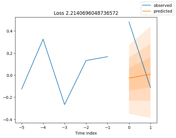
[ ]: