使用时间融合变压器进行需求预测#

在本教程中，我们将在非常小的数据集上训练TemporalFusionTransformer，以展示即使在仅有20k样本的情况下，它也能表现出色。一般来说，这是一个大型模型，因此在更多数据的情况下表现会更好。

我们的示例是来自Stallion kaggle竞赛的需求预测。

[1]:

import warnings

warnings.filterwarnings("ignore")  # avoid printing out absolute paths

[2]:

import copy
from pathlib import Path
import warnings

import lightning.pytorch as pl
from lightning.pytorch.callbacks import EarlyStopping, LearningRateMonitor
from lightning.pytorch.loggers import TensorBoardLogger
import numpy as np
import pandas as pd
import torch

from pytorch_forecasting import Baseline, TemporalFusionTransformer, TimeSeriesDataSet
from pytorch_forecasting.data import GroupNormalizer
from pytorch_forecasting.metrics import MAE, SMAPE, PoissonLoss, QuantileLoss
from pytorch_forecasting.models.temporal_fusion_transformer.tuning import (
    optimize_hyperparameters,
)

加载数据#

首先，我们需要将我们的时间序列转换为一个pandas数据框，其中每一行都可以通过时间步长和时间序列来识别。幸运的是，大多数数据集已经采用这种格式。在本教程中，我们将使用Kaggle上的Stallion数据集，该数据集描述了各种饮料的销售情况。我们的任务是通过库存单位（SKU），即产品，由代理商（即商店）销售，进行六个月的销售量预测。大约有21,000条月度历史销售记录。除了历史销售数据外，我们还有关于销售价格、代理商位置、特殊日子（如假期）以及整个行业的销售量的信息。

数据集已经处于正确的格式，但缺少一些重要的特征。最重要的是，我们需要添加一个时间索引，每个时间步长递增一次。此外，添加日期特征是有益的，在这种情况下意味着从日期记录中提取月份。

[3]:

from pytorch_forecasting.data.examples import get_stallion_data

data = get_stallion_data()

# add time index
data["time_idx"] = data["date"].dt.year * 12 + data["date"].dt.month
data["time_idx"] -= data["time_idx"].min()

# add additional features
data["month"] = data.date.dt.month.astype(str).astype(
    "category"
)  # categories have be strings
data["log_volume"] = np.log(data.volume + 1e-8)
data["avg_volume_by_sku"] = data.groupby(
    ["time_idx", "sku"], observed=True
).volume.transform("mean")
data["avg_volume_by_agency"] = data.groupby(
    ["time_idx", "agency"], observed=True
).volume.transform("mean")

# we want to encode special days as one variable and thus need to first reverse one-hot encoding
special_days = [
    "easter_day",
    "good_friday",
    "new_year",
    "christmas",
    "labor_day",
    "independence_day",
    "revolution_day_memorial",
    "regional_games",
    "fifa_u_17_world_cup",
    "football_gold_cup",
    "beer_capital",
    "music_fest",
]
data[special_days] = (
    data[special_days].apply(lambda x: x.map({0: "-", 1: x.name})).astype("category")
)
data.sample(10, random_state=521)

[3]:

	机构	库存单位	销量	日期	行业销量	苏打水销量	平均最高温度	常规价格	实际价格	折扣	...	足球金杯	啤酒之都	音乐节	折扣百分比	时间序列	时间索引	月份	对数销量	按库存单位的平均销量	按机构的平均销量
291	代理_25	SKU_03	0.5076	2013-01-01	492612703	718394219	25.845238	1264.162234	1152.473405	111.688829	...	-	-	-	8.835008	228	0	1	-0.678062	1225.306376	99.650400
871	代理机构_29	SKU_02	8.7480	2015-01-01	498567142	762225057	27.584615	1316.098485	1296.804924	19.293561	...	-	-	-	1.465966	177	24	1	2.168825	1634.434615	11.397086
19532	代理机构_47	SKU_01	4.9680	2013-09-01	454252482	789624076	30.665957	1269.250000	1266.490490	2.759510	...	-	-	-	0.217413	322	8	9	1.603017	2625.472644	48.295650
2089	Agency_53	SKU_07	21.6825	2013-10-01	480693900	791658684	29.197727	1193.842373	1128.124395	65.717978	...	-	啤酒之都	-	5.504745	240	9	10	3.076505	38.529107	2511.035175
9755	Agency_17	SKU_02	960.5520	2015-03-01	515468092	871204688	23.608120	1338.334248	1232.128069	106.206179	...	-	-	音乐节	7.935699	259	26	3	6.867508	2143.677462	396.022140
7561	Agency_05	SKU_03	1184.6535	2014-02-01	425528909	734443953	28.668254	1369.556376	1161.135214	208.421162	...	-	-	-	15.218151	21	13	2	7.077206	1566.643589	1881.866367
19204	Agency_11	SKU_05	5.5593	2017-08-01	623319783	1049868815	31.915385	1922.486644	1651.307674	271.178970	...	-	-	-	14.105636	17	55	8	1.715472	1385.225478	109.699200
8781	Agency_48	SKU_04	4275.1605	2013-03-01	509281531	892192092	26.767857	1761.258209	1546.059670	215.198539	...	-	-	音乐节	12.218455	151	2	3	8.360577	1757.950603	1925.272108
2540	Agency_07	SKU_21	0.0000	2015-10-01	544203593	761469815	28.987755	0.000000	0.000000	0.000000	...	-	-	-	0.000000	300	33	10	-18.420681	0.000000	2418.719550
12084	Agency_21	SKU_03	46.3608	2017-04-01	589969396	940912941	32.478910	1675.922116	1413.571789	262.350327	...	-	-	-	15.654088	181	51	4	3.836454	2034.293024	109.381800

10 行 × 31 列

[4]:

data.describe()

[4]:

	体积	日期	行业体积	苏打体积	平均最高温度	常规价格	实际价格	折扣	2017年平均人口	2017年平均家庭年收入	折扣百分比	时间序列	时间索引	对数体积	按SKU的平均体积	按代理的平均体积
计数	21000.000000	21000	2.100000e+04	2.100000e+04	21000.000000	21000.000000	21000.000000	21000.000000	2.100000e+04	21000.000000	21000.000000	21000.00000	21000.000000	21000.000000	21000.000000	21000.000000
平均值	1492.403982	2015-06-16 20:48:00	5.439214e+08	8.512000e+08	28.612404	1451.536344	1267.347450	184.374146	1.045065e+06	151073.494286	10.574884	174.50000	29.500000	2.464118	1492.403982	1492.403982
最小值	0.000000	2013-01-01 00:00:00	4.130518e+08	6.964015e+08	16.731034	0.000000	-3121.690141	0.000000	1.227100e+04	90240.000000	0.000000	0.00000	0.000000	-18.420681	0.000000	0.000000
25%	8.272388	2014-03-24 06:00:00	5.090553e+08	7.890880e+08	25.374816	1311.547158	1178.365653	54.935108	6.018900e+04	110057.000000	3.749628	87.00000	14.750000	2.112923	932.285496	113.420250
50%	158.436000	2015-06-16 00:00:00	5.512000e+08	8.649196e+08	28.479272	1495.174592	1324.695705	138.307225	1.232242e+06	131411.000000	8.948990	174.50000	29.500000	5.065351	1402.305264	1730.529771
75%	1774.793475	2016-09-08 12:00:00	5.893715e+08	9.005551e+08	31.568405	1725.652080	1517.311427	272.298630	1.729177e+06	206553.000000	15.647058	262.00000	44.250000	7.481439	2195.362302	2595.316500
最大值	22526.610000	2017-12-01 00:00:00	6.700157e+08	1.049869e+09	45.290476	19166.625000	4925.404000	19166.625000	3.137874e+06	247220.000000	226.740147	349.00000	59.000000	10.022453	4332.363750	5884.717375
标准差	2711.496882	NaN	6.288022e+07	7.824340e+07	3.972833	683.362417	587.757323	257.469968	9.291926e+05	50409.593114	9.590813	101.03829	17.318515	8.178218	1051.790829	1328.239698

创建数据集和数据加载器#

下一步是将数据框转换为PyTorch Forecasting的TimeSeriesDataSet。除了告诉数据集哪些特征是分类的与连续的，哪些是静态的与随时间变化的，我们还需要决定如何对数据进行归一化。在这里，我们分别对每个时间序列进行标准缩放，并指示值始终为正。通常，EncoderNormalizer在训练时动态缩放每个编码器序列，以避免归一化引起的前瞻性偏差。然而，如果你在寻找一个相对稳定的归一化方法时遇到困难，例如因为数据中有很多零，或者你期望在推理时有一个更稳定的归一化，你可能会接受前瞻性偏差。在后一种情况下，你可以确保不会学习到在运行推理时不会出现的“奇怪”跳跃，从而在一个更现实的数据集上进行训练。

我们还选择使用最后六个月作为验证集。

[5]:

max_prediction_length = 6
max_encoder_length = 24
training_cutoff = data["time_idx"].max() - max_prediction_length

training = TimeSeriesDataSet(
    data[lambda x: x.time_idx <= training_cutoff],
    time_idx="time_idx",
    target="volume",
    group_ids=["agency", "sku"],
    min_encoder_length=max_encoder_length
    // 2,  # keep encoder length long (as it is in the validation set)
    max_encoder_length=max_encoder_length,
    min_prediction_length=1,
    max_prediction_length=max_prediction_length,
    static_categoricals=["agency", "sku"],
    static_reals=["avg_population_2017", "avg_yearly_household_income_2017"],
    time_varying_known_categoricals=["special_days", "month"],
    variable_groups={
        "special_days": special_days
    },  # group of categorical variables can be treated as one variable
    time_varying_known_reals=["time_idx", "price_regular", "discount_in_percent"],
    time_varying_unknown_categoricals=[],
    time_varying_unknown_reals=[
        "volume",
        "log_volume",
        "industry_volume",
        "soda_volume",
        "avg_max_temp",
        "avg_volume_by_agency",
        "avg_volume_by_sku",
    ],
    target_normalizer=GroupNormalizer(
        groups=["agency", "sku"], transformation="softplus"
    ),  # use softplus and normalize by group
    add_relative_time_idx=True,
    add_target_scales=True,
    add_encoder_length=True,
)

# create validation set (predict=True) which means to predict the last max_prediction_length points in time
# for each series
validation = TimeSeriesDataSet.from_dataset(
    training, data, predict=True, stop_randomization=True
)

# create dataloaders for model
batch_size = 128  # set this between 32 to 128
train_dataloader = training.to_dataloader(
    train=True, batch_size=batch_size, num_workers=0
)
val_dataloader = validation.to_dataloader(
    train=False, batch_size=batch_size * 10, num_workers=0
)

要了解更多关于TimeSeriesDataSet的信息，请访问其文档或解释如何将数据集传递给模型的教程。

创建基线模型#

评估一个Baseline模型，该模型通过简单地重复最后观察到的量来预测接下来的6个月，为我们提供了一个我们希望超越的简单基准。

[6]:

# calculate baseline mean absolute error, i.e. predict next value as the last available value from the history
baseline_predictions = Baseline().predict(val_dataloader, return_y=True)
MAE()(baseline_predictions.output, baseline_predictions.y)

GPU available: True (mps), used: True
TPU available: False, using: 0 TPU cores
HPU available: False, using: 0 HPUs

[6]:

tensor(293.0089, device='mps:0')

训练时间融合变压器#

现在是时候创建我们的TemporalFusionTransformer模型了。我们使用PyTorch Lightning来训练模型。

找到最佳学习率#

在训练之前，您可以使用PyTorch Lightning学习率查找器来识别最佳学习率。

[7]:

# configure network and trainer
pl.seed_everything(42)
trainer = pl.Trainer(
    accelerator="cpu",
    # clipping gradients is a hyperparameter and important to prevent divergance
    # of the gradient for recurrent neural networks
    gradient_clip_val=0.1,
)


tft = TemporalFusionTransformer.from_dataset(
    training,
    # not meaningful for finding the learning rate but otherwise very important
    learning_rate=0.03,
    hidden_size=8,  # most important hyperparameter apart from learning rate
    # number of attention heads. Set to up to 4 for large datasets
    attention_head_size=1,
    dropout=0.1,  # between 0.1 and 0.3 are good values
    hidden_continuous_size=8,  # set to <= hidden_size
    loss=QuantileLoss(),
    optimizer="ranger",
    # reduce learning rate if no improvement in validation loss after x epochs
    # reduce_on_plateau_patience=1000,
)
print(f"Number of parameters in network: {tft.size() / 1e3:.1f}k")

Seed set to 42
GPU available: True (mps), used: False
TPU available: False, using: 0 TPU cores
HPU available: False, using: 0 HPUs

Number of parameters in network: 13.5k

[8]:

# find optimal learning rate
from lightning.pytorch.tuner import Tuner

res = Tuner(trainer).lr_find(
    tft,
    train_dataloaders=train_dataloader,
    val_dataloaders=val_dataloader,
    max_lr=10.0,
    min_lr=1e-6,
)

print(f"suggested learning rate: {res.suggestion()}")
fig = res.plot(show=True, suggest=True)
fig.show()

`Trainer.fit` stopped: `max_steps=100` reached.
Learning rate set to 0.0097723722095581
Restoring states from the checkpoint path at /Users/hirwa/Desktop/open/for/pytorch-forecasting/docs/source/tutorials/.lr_find_9962a241-9a34-45b4-b4b4-5fae485145c7.ckpt
Restored all states from the checkpoint at /Users/hirwa/Desktop/open/for/pytorch-forecasting/docs/source/tutorials/.lr_find_9962a241-9a34-45b4-b4b4-5fae485145c7.ckpt

suggested learning rate: 0.0097723722095581

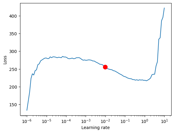
对于TemporalFusionTransformer，最佳学习率似乎略低于建议的学习率。此外，我们不想直接使用建议的学习率，因为PyTorch Lightning有时会被较低学习率下的噪声所迷惑，并建议过低的学习率。手动控制是必要的。我们决定选择0.03作为学习率。

训练模型#

如果您在训练模型时遇到问题并出现错误 AttributeError: module 'tensorflow._api.v2.io.gfile' has no attribute 'get_filesystem'，请考虑卸载 tensorflow 或首先执行

import tensorflow as tf
import tensorboard as tb
tf.io.gfile = tb.compat.tensorflow_stub.io.gfile
```.

[9]:

# configure network and trainer
early_stop_callback = EarlyStopping(
    monitor="val_loss", min_delta=1e-4, patience=10, verbose=False, mode="min"
)
lr_logger = LearningRateMonitor()  # log the learning rate
logger = TensorBoardLogger("lightning_logs")  # logging results to a tensorboard

trainer = pl.Trainer(
    max_epochs=50,
    accelerator="cpu",
    enable_model_summary=True,
    gradient_clip_val=0.1,
    limit_train_batches=50,  # coment in for training, running valiation every 30 batches
    # fast_dev_run=True,  # comment in to check that networkor dataset has no serious bugs
    callbacks=[lr_logger, early_stop_callback],
    logger=logger,
)

tft = TemporalFusionTransformer.from_dataset(
    training,
    learning_rate=0.03,
    hidden_size=16,
    attention_head_size=2,
    dropout=0.1,
    hidden_continuous_size=8,
    loss=QuantileLoss(),
    log_interval=10,  # uncomment for learning rate finder and otherwise, e.g. to 10 for logging every 10 batches
    optimizer="ranger",
    reduce_on_plateau_patience=4,
)
print(f"Number of parameters in network: {tft.size() / 1e3:.1f}k")

GPU available: True (mps), used: False
TPU available: False, using: 0 TPU cores
HPU available: False, using: 0 HPUs

Number of parameters in network: 29.4k

在我的Macbook上训练需要几分钟，但对于更大的网络和数据集，可能需要几个小时。训练速度主要取决于开销，选择更大的batch_size或hidden_size（即网络大小）不会线性地减慢训练速度，使得在大数据集上进行训练成为可能。在训练过程中，我们可以监控tensorboard，可以通过tensorboard --logdir=lightning_logs启动。例如，我们可以监控训练集和验证集上的预测示例。

[10]:

# fit network
trainer.fit(
    tft,
    train_dataloaders=train_dataloader,
    val_dataloaders=val_dataloader,
)


   | Name                               | Type                            | Params | Mode
------------------------------------------------------------------------------------------------
0  | loss                               | QuantileLoss                    | 0      | train
1  | logging_metrics                    | ModuleList                      | 0      | train
2  | input_embeddings                   | MultiEmbedding                  | 1.3 K  | train
3  | prescalers                         | ModuleDict                      | 256    | train
4  | static_variable_selection          | VariableSelectionNetwork        | 3.4 K  | train
5  | encoder_variable_selection         | VariableSelectionNetwork        | 8.0 K  | train
6  | decoder_variable_selection         | VariableSelectionNetwork        | 2.7 K  | train
7  | static_context_variable_selection  | GatedResidualNetwork            | 1.1 K  | train
8  | static_context_initial_hidden_lstm | GatedResidualNetwork            | 1.1 K  | train
9  | static_context_initial_cell_lstm   | GatedResidualNetwork            | 1.1 K  | train
10 | static_context_enrichment          | GatedResidualNetwork            | 1.1 K  | train
11 | lstm_encoder                       | LSTM                            | 2.2 K  | train
12 | lstm_decoder                       | LSTM                            | 2.2 K  | train
13 | post_lstm_gate_encoder             | GatedLinearUnit                 | 544    | train
14 | post_lstm_add_norm_encoder         | AddNorm                         | 32     | train
15 | static_enrichment                  | GatedResidualNetwork            | 1.4 K  | train
16 | multihead_attn                     | InterpretableMultiHeadAttention | 808    | train
17 | post_attn_gate_norm                | GateAddNorm                     | 576    | train
18 | pos_wise_ff                        | GatedResidualNetwork            | 1.1 K  | train
19 | pre_output_gate_norm               | GateAddNorm                     | 576    | train
20 | output_layer                       | Linear                          | 119    | train
------------------------------------------------------------------------------------------------
29.4 K    Trainable params
0         Non-trainable params
29.4 K    Total params
0.118     Total estimated model params size (MB)
480       Modules in train mode
0         Modules in eval mode

`Trainer.fit` stopped: `max_epochs=50` reached.

超参数调优#

使用[optuna](https://optuna.org/)进行超参数调优直接集成在pytorch-forecasting中。例如，我们可以使用 optimize_hyperparameters()函数来优化TFT的超参数。

import pickle

from pytorch_forecasting.models.temporal_fusion_transformer.tuning import optimize_hyperparameters

# create study
study = optimize_hyperparameters(
    train_dataloader,
    val_dataloader,
    model_path="optuna_test",
    n_trials=200,
    max_epochs=50,
    gradient_clip_val_range=(0.01, 1.0),
    hidden_size_range=(8, 128),
    hidden_continuous_size_range=(8, 128),
    attention_head_size_range=(1, 4),
    learning_rate_range=(0.001, 0.1),
    dropout_range=(0.1, 0.3),
    trainer_kwargs=dict(limit_train_batches=30),
    reduce_on_plateau_patience=4,
    use_learning_rate_finder=False,  # use Optuna to find ideal learning rate or use in-built learning rate finder
)

# save study results - also we can resume tuning at a later point in time
with open("test_study.pkl", "wb") as fout:
    pickle.dump(study, fout)

# show best hyperparameters
print(study.best_trial.params)

评估性能#

PyTorch Lightning 自动检查点训练，因此我们可以轻松检索最佳模型并加载它。

[11]:

# load the best model according to the validation loss
# (given that we use early stopping, this is not necessarily the last epoch)
best_model_path = trainer.checkpoint_callback.best_model_path
best_tft = TemporalFusionTransformer.load_from_checkpoint(best_model_path)

训练后，我们可以使用predict()进行预测。该方法允许对其返回的内容进行非常精细的控制，例如，您可以轻松地将预测与您的pandas数据框匹配。详情请参阅其文档。我们在验证数据集和一些示例上评估指标，以查看模型的表现如何。鉴于我们仅使用21,000个样本，结果非常令人放心，并且可以与梯度提升器的结果竞争。我们的表现也优于基线模型。考虑到数据的噪声，这并非易事。

[12]:

# calcualte mean absolute error on validation set
predictions = best_tft.predict(
    val_dataloader, return_y=True, trainer_kwargs=dict(accelerator="cpu")
)
MAE()(predictions.output, predictions.y)

GPU available: True (mps), used: False
TPU available: False, using: 0 TPU cores
HPU available: False, using: 0 HPUs

[12]:

tensor(359.3377)

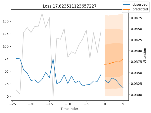
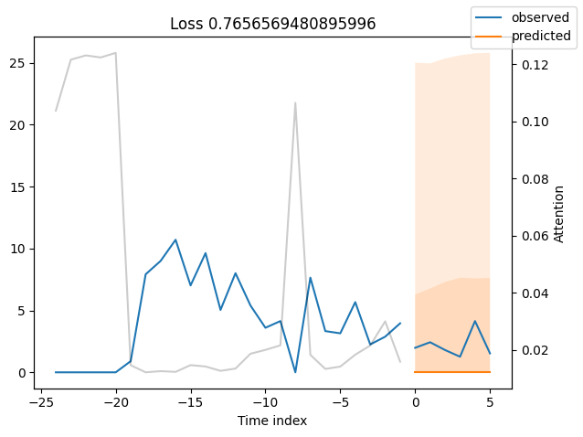
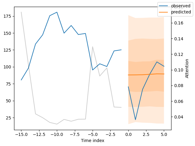
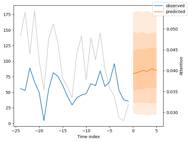
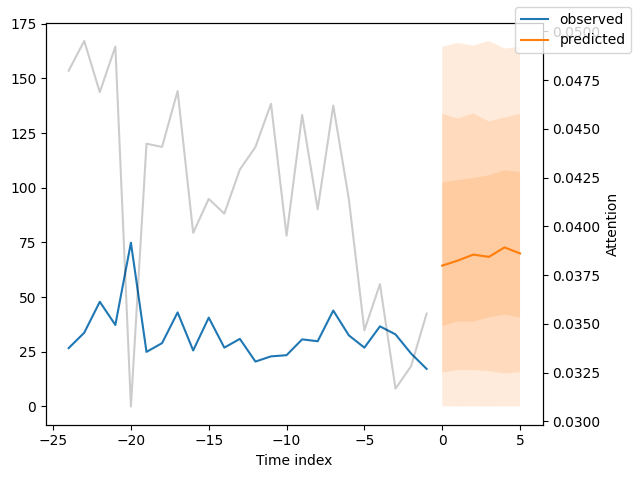
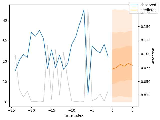
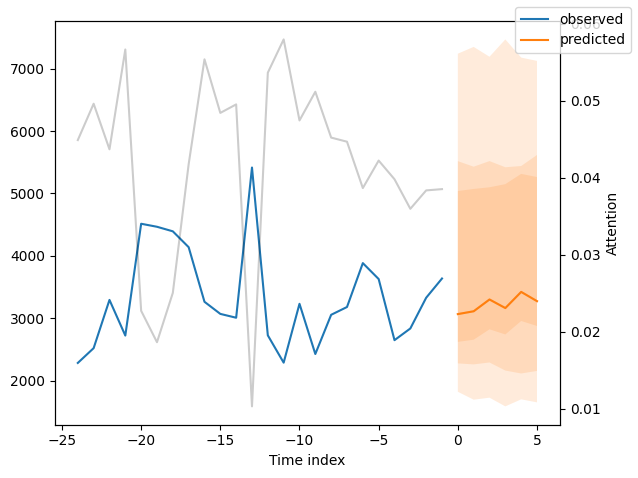
我们现在也可以直接查看样本预测，我们使用plot_prediction()进行绘制。正如你从下面的图表中看到的，预测看起来相当准确。如果你想知道，灰色线条表示模型在进行预测时对不同时间点的关注程度。这是时间融合变压器的一个特殊功能。

[13]:

# raw predictions are a dictionary from which all kind of information including quantiles can be extracted
raw_predictions = best_tft.predict(
    val_dataloader, mode="raw", return_x=True, trainer_kwargs=dict(accelerator="cpu")
)

GPU available: True (mps), used: False
TPU available: False, using: 0 TPU cores
HPU available: False, using: 0 HPUs

[14]:

for idx in range(10):  # plot 10 examples
    best_tft.plot_prediction(
        raw_predictions.x, raw_predictions.output, idx=idx, add_loss_to_title=True
    )

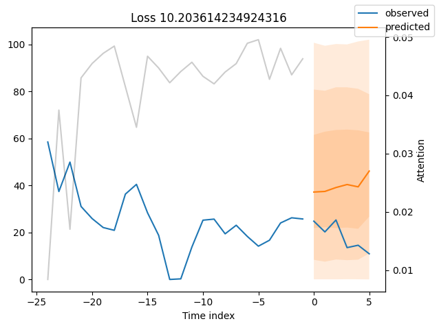
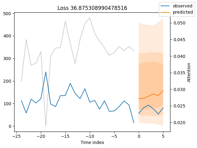
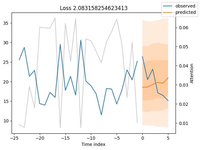
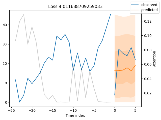
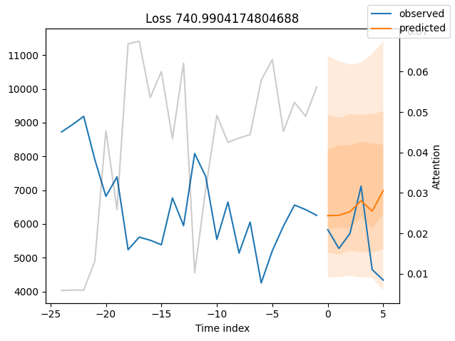
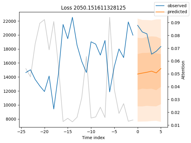
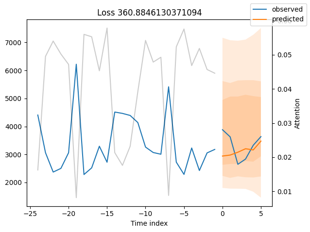
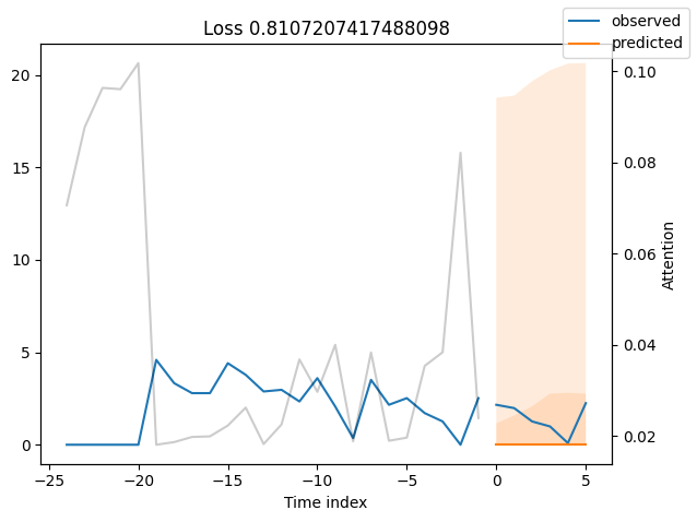
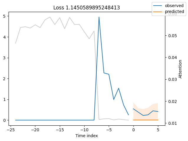
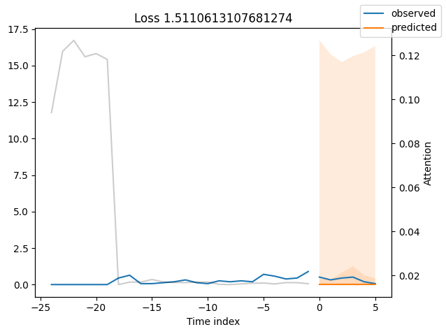
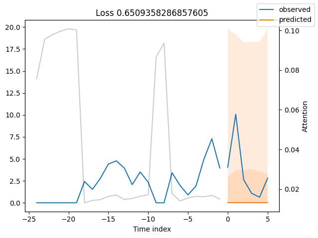
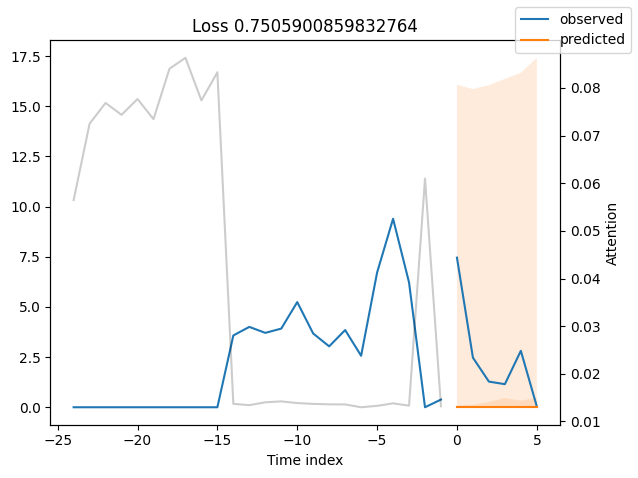
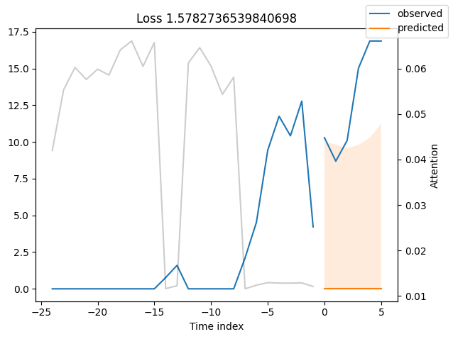
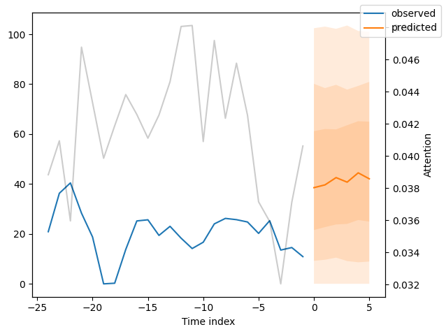
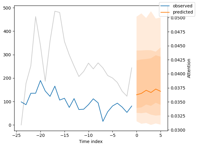
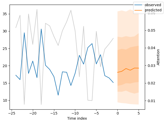
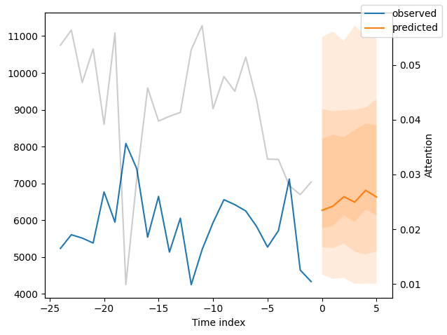
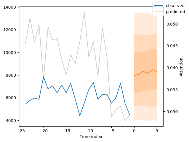
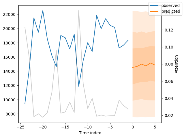
表现最差#

观察表现最差的模型，例如在SMAPE方面，可以让我们了解模型在可靠预测方面存在的问题。这些例子可以提供关于如何改进模型的重要线索。这种实际值与预测值的对比图对所有模型都可用。当然，使用额外的指标也是明智的，例如在metrics模块中定义的MASE。然而，为了演示的目的，我们在这里只使用SMAPE。

[15]:

# calcualte metric by which to display
predictions = best_tft.predict(
    val_dataloader, return_y=True, trainer_kwargs=dict(accelerator="cpu")
)
mean_losses = SMAPE(reduction="none").loss(predictions.output, predictions.y[0]).mean(1)
indices = mean_losses.argsort(descending=True)  # sort losses
for idx in range(10):  # plot 10 examples
    best_tft.plot_prediction(
        raw_predictions.x,
        raw_predictions.output,
        idx=indices[idx],
        add_loss_to_title=SMAPE(quantiles=best_tft.loss.quantiles),
    )

GPU available: True (mps), used: False
TPU available: False, using: 0 TPU cores
HPU available: False, using: 0 HPUs

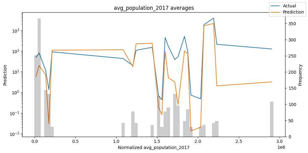
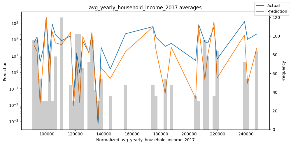
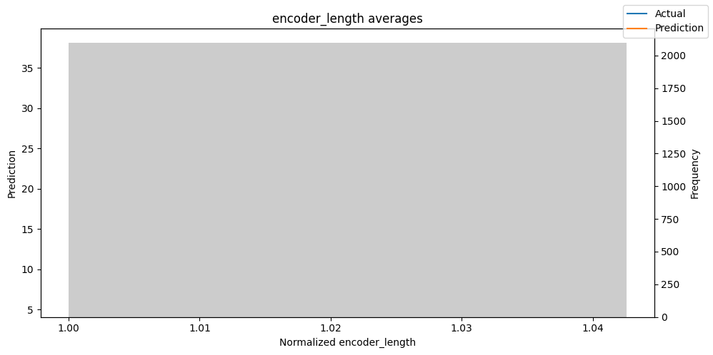
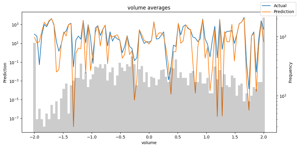
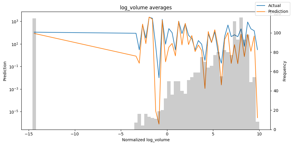
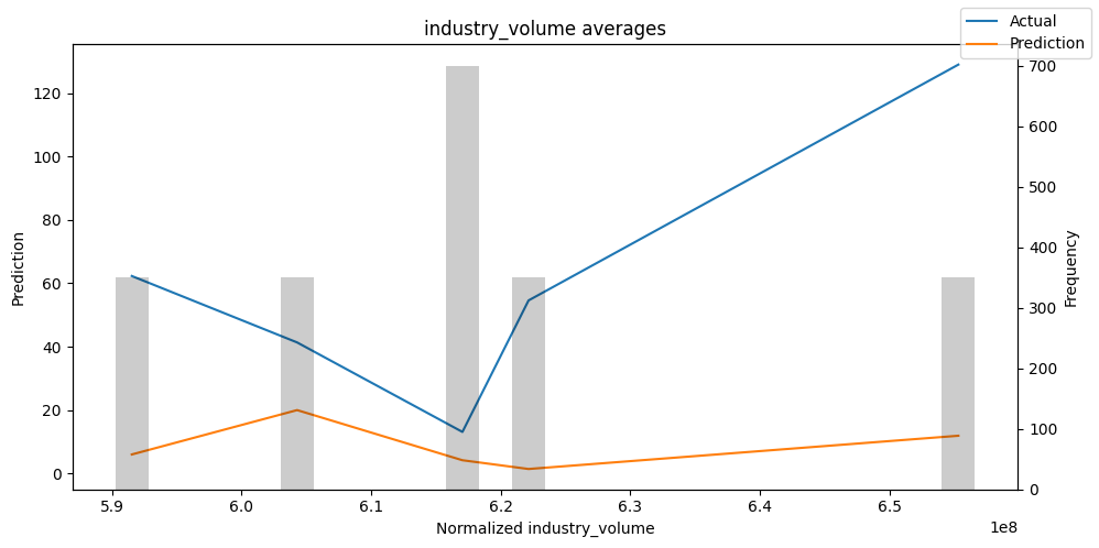
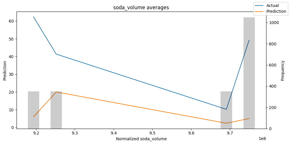
按变量的实际值与预测值#

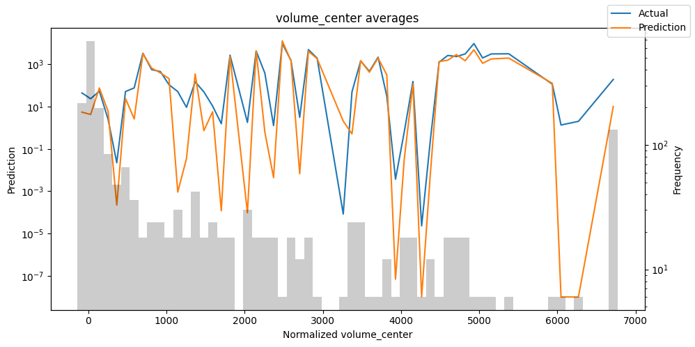
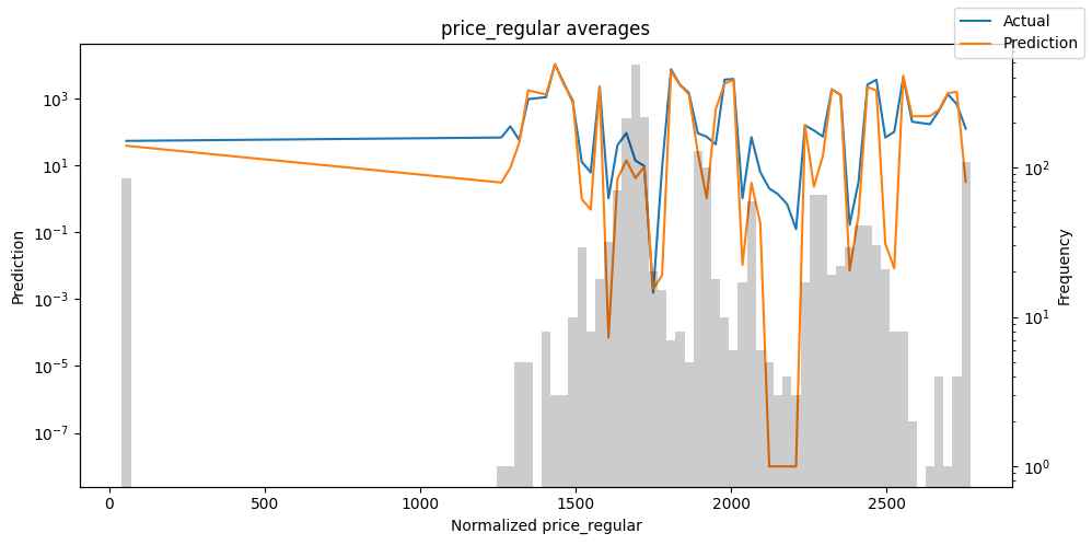
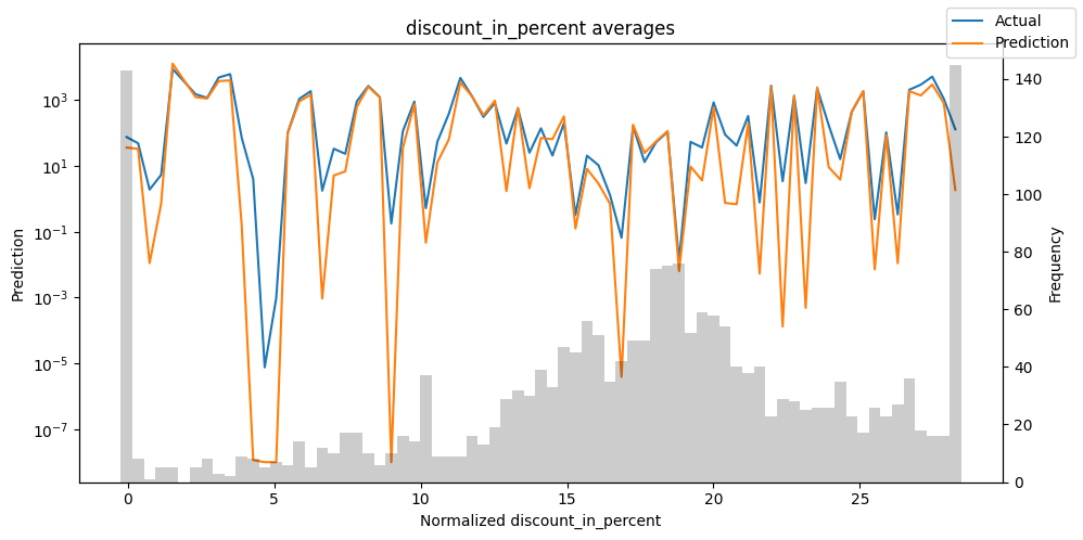
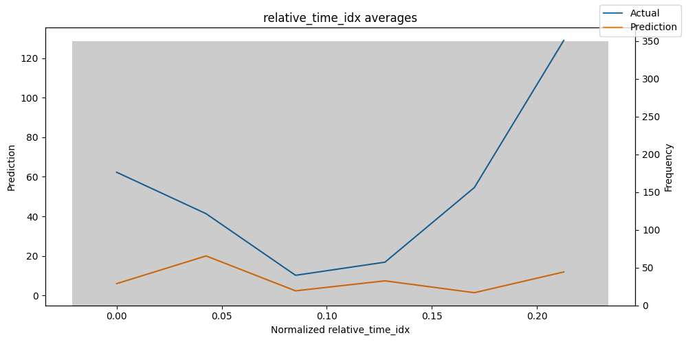
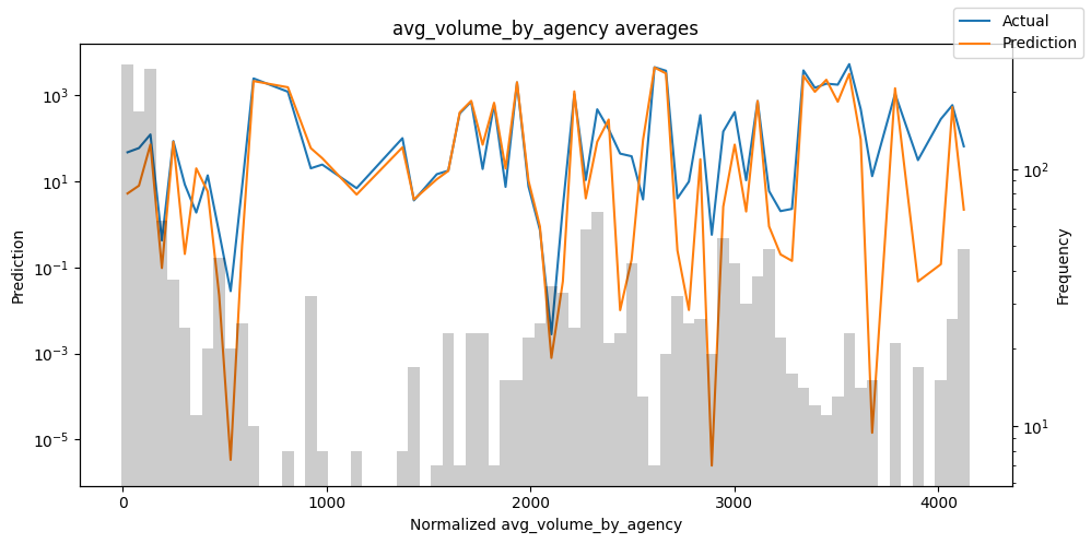
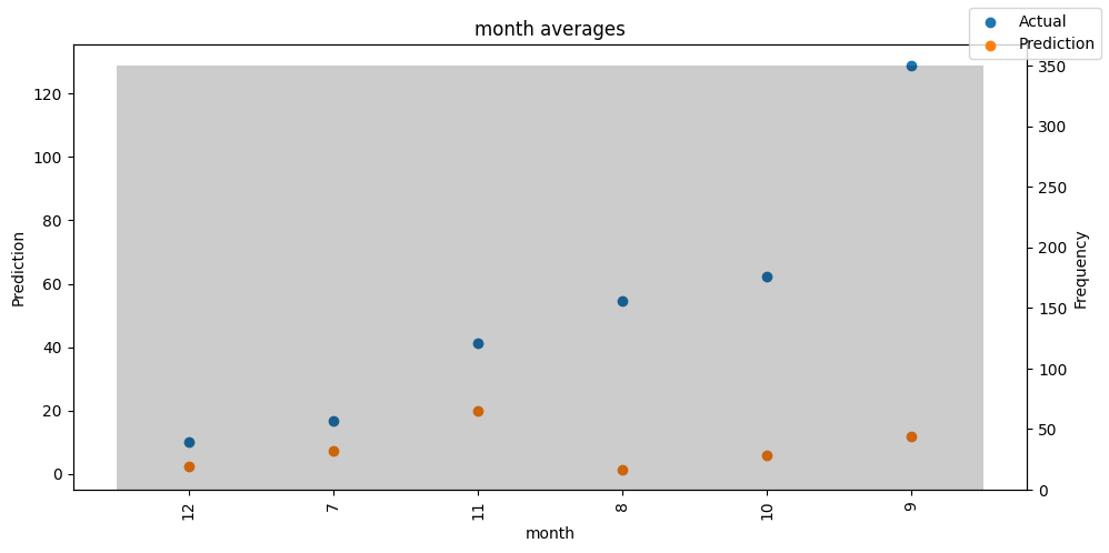
检查模型在不同数据切片上的表现可以帮助我们发现弱点。下面绘制的是每个变量分成100个区间后预测值与实际值的均值。现在，我们可以直接使用calculate_prediction_actual_by_variable()和plot_prediction_actual_by_variable()方法对生成的数据进行预测。灰色条表示每个区间的变量频率，即直方图。

[16]:

predictions = best_tft.predict(
    val_dataloader, return_x=True, trainer_kwargs=dict(accelerator="cpu")
)
predictions_vs_actuals = best_tft.calculate_prediction_actual_by_variable(
    predictions.x, predictions.output
)
best_tft.plot_prediction_actual_by_variable(predictions_vs_actuals)

GPU available: True (mps), used: False
TPU available: False, using: 0 TPU cores
HPU available: False, using: 0 HPUs

[16]:

{'avg_population_2017': <Figure size 1000x500 with 2 Axes>,
 'avg_yearly_household_income_2017': <Figure size 1000x500 with 2 Axes>,
 'encoder_length': <Figure size 1000x500 with 2 Axes>,
 'volume_center': <Figure size 1000x500 with 2 Axes>,
 'volume_scale': <Figure size 1000x500 with 2 Axes>,
 'time_idx': <Figure size 1000x500 with 2 Axes>,
 'price_regular': <Figure size 1000x500 with 2 Axes>,
 'discount_in_percent': <Figure size 1000x500 with 2 Axes>,
 'relative_time_idx': <Figure size 1000x500 with 2 Axes>,
 'volume': <Figure size 1000x500 with 2 Axes>,
 'log_volume': <Figure size 1000x500 with 2 Axes>,
 'industry_volume': <Figure size 1000x500 with 2 Axes>,
 'soda_volume': <Figure size 1000x500 with 2 Axes>,
 'avg_max_temp': <Figure size 1000x500 with 2 Axes>,
 'avg_volume_by_agency': <Figure size 1000x500 with 2 Axes>,
 'avg_volume_by_sku': <Figure size 1000x500 with 2 Axes>,
 'agency': <Figure size 1000x500 with 2 Axes>,
 'sku': <Figure size 1000x500 with 2 Axes>,
 'special_days': <Figure size 1000x500 with 2 Axes>,
 'month': <Figure size 1000x500 with 2 Axes>}

预测选定的数据#

为了预测数据的子集，我们可以使用filter()方法过滤数据集中的子序列。这里我们预测training数据集中映射到组ID“Agency_01”和“SKU_01”且第一个预测值对应时间索引“15”的子序列。我们输出所有七个分位数。这意味着我们期望得到一个形状为1 x n_timesteps x n_quantiles = 1 x 6 x 7的张量，因为我们预测单个子序列的六个时间步长，并且每个时间步长有7个分位数。

[17]:

best_tft.predict(
    training.filter(
        lambda x: (x.agency == "Agency_01")
        & (x.sku == "SKU_01")
        & (x.time_idx_first_prediction == 15)
    ),
    mode="quantiles",
    trainer_kwargs=dict(accelerator="cpu"),
)

GPU available: True (mps), used: False
TPU available: False, using: 0 TPU cores
HPU available: False, using: 0 HPUs

[17]:

tensor([[[ 15.4090,  40.9870,  64.1208,  88.0738, 108.6642, 138.7954, 176.3737],
         [ 18.3478,  40.8236,  62.9533,  88.1478, 107.2123, 141.3340, 172.1918],
         [ 17.5609,  41.0912,  63.2938,  88.3589, 107.9875, 141.8121, 172.3604],
         [ 17.2089,  41.6997,  63.6379,  88.9980, 108.1090, 141.3753, 172.8454],
         [ 16.3293,  40.8779,  64.4161,  89.6760, 110.5591, 141.1115, 172.8432],
         [ 16.1977,  40.8351,  63.3174,  89.5182, 110.2483, 141.9060, 173.6944]]])

当然，我们也可以轻松地绘制这个预测：

[18]:

raw_prediction = best_tft.predict(
    training.filter(
        lambda x: (x.agency == "Agency_01")
        & (x.sku == "SKU_01")
        & (x.time_idx_first_prediction == 15)
    ),
    mode="raw",
    return_x=True,
    trainer_kwargs=dict(accelerator="cpu"),
)
best_tft.plot_prediction(raw_prediction.x, raw_prediction.output, idx=0)

GPU available: True (mps), used: False
TPU available: False, using: 0 TPU cores
HPU available: False, using: 0 HPUs

[18]:

预测新数据#

因为我们在数据集中有协变量，预测新数据需要我们预先定义已知的协变量。

[19]:

# select last 24 months from data (max_encoder_length is 24)
encoder_data = data[lambda x: x.time_idx > x.time_idx.max() - max_encoder_length]

# select last known data point and create decoder data from it by repeating it and incrementing the month
# in a real world dataset, we should not just forward fill the covariates but specify them to account
# for changes in special days and prices (which you absolutely should do but we are too lazy here)
last_data = data[lambda x: x.time_idx == x.time_idx.max()]
decoder_data = pd.concat(
    [
        last_data.assign(date=lambda x: x.date + pd.offsets.MonthBegin(i))
        for i in range(1, max_prediction_length + 1)
    ],
    ignore_index=True,
)

# add time index consistent with "data"
decoder_data["time_idx"] = (
    decoder_data["date"].dt.year * 12 + decoder_data["date"].dt.month
)
decoder_data["time_idx"] += (
    encoder_data["time_idx"].max() + 1 - decoder_data["time_idx"].min()
)

# adjust additional time feature(s)
decoder_data["month"] = decoder_data.date.dt.month.astype(str).astype(
    "category"
)  # categories have be strings

# combine encoder and decoder data
new_prediction_data = pd.concat([encoder_data, decoder_data], ignore_index=True)

现在，我们可以直接使用predict()方法对生成的数据进行预测。

[20]:

new_raw_predictions = best_tft.predict(
    new_prediction_data,
    mode="raw",
    return_x=True,
    trainer_kwargs=dict(accelerator="cpu"),
)

for idx in range(10):  # plot 10 examples
    best_tft.plot_prediction(
        new_raw_predictions.x,
        new_raw_predictions.output,
        idx=idx,
        show_future_observed=False,
    )

GPU available: True (mps), used: False
TPU available: False, using: 0 TPU cores
HPU available: False, using: 0 HPUs

解释模型#

变量重要性#

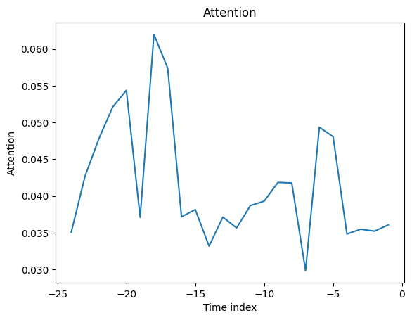
该模型由于其架构的构建方式，具有内置的解释能力。让我们看看这是如何表现的。我们首先使用interpret_output()计算解释，然后使用plot_interpretation()绘制它们。

[21]:

interpretation = best_tft.interpret_output(raw_predictions.output, reduction="sum")
best_tft.plot_interpretation(interpretation)

[21]:

{'attention': <Figure size 640x480 with 1 Axes>,
 'static_variables': <Figure size 700x375 with 1 Axes>,
 'encoder_variables': <Figure size 700x525 with 1 Axes>,
 'decoder_variables': <Figure size 700x350 with 1 Axes>}

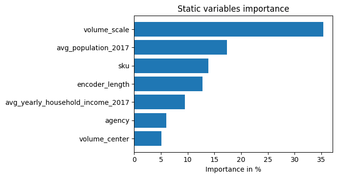
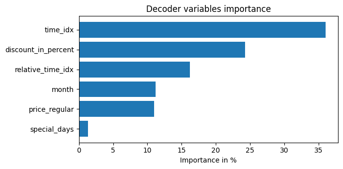
不出所料，过去观察到的交易量特征是编码器中的首要变量，而与价格相关的变量是解码器中的主要预测因素。

一般的注意力模式似乎是最近的观察更为重要，而较旧的观察则不那么重要。这证实了直觉。平均注意力通常不太有用——通过示例查看注意力更有洞察力，因为模式不会被平均化。

部分依赖#

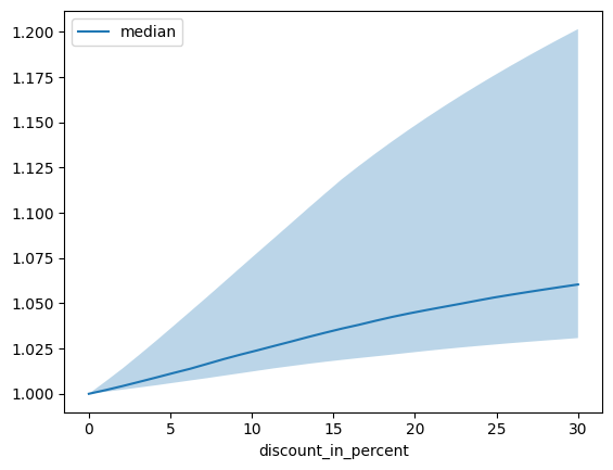
部分依赖图通常用于更好地解释模型（假设特征独立）。它们也可以用于理解在模拟情况下可以预期什么，并且是使用predict_dependency()创建的。

[22]:

dependency = best_tft.predict_dependency(
    val_dataloader.dataset,
    "discount_in_percent",
    np.linspace(0, 30, 30),
    show_progress_bar=True,
    mode="dataframe",
    trainer_kwargs=dict(accelerator="cpu"),
)

GPU available: True (mps), used: False
TPU available: False, using: 0 TPU cores
HPU available: False, using: 0 HPUs
GPU available: True (mps), used: False
TPU available: False, using: 0 TPU cores
HPU available: False, using: 0 HPUs
GPU available: True (mps), used: False
TPU available: False, using: 0 TPU cores
HPU available: False, using: 0 HPUs
GPU available: True (mps), used: False
TPU available: False, using: 0 TPU cores
HPU available: False, using: 0 HPUs
GPU available: True (mps), used: False
TPU available: False, using: 0 TPU cores
HPU available: False, using: 0 HPUs
GPU available: True (mps), used: False
TPU available: False, using: 0 TPU cores
HPU available: False, using: 0 HPUs
GPU available: True (mps), used: False
TPU available: False, using: 0 TPU cores
HPU available: False, using: 0 HPUs
GPU available: True (mps), used: False
TPU available: False, using: 0 TPU cores
HPU available: False, using: 0 HPUs
GPU available: True (mps), used: False
TPU available: False, using: 0 TPU cores
HPU available: False, using: 0 HPUs
GPU available: True (mps), used: False
TPU available: False, using: 0 TPU cores
HPU available: False, using: 0 HPUs
GPU available: True (mps), used: False
TPU available: False, using: 0 TPU cores
HPU available: False, using: 0 HPUs
GPU available: True (mps), used: False
TPU available: False, using: 0 TPU cores
HPU available: False, using: 0 HPUs
GPU available: True (mps), used: False
TPU available: False, using: 0 TPU cores
HPU available: False, using: 0 HPUs
GPU available: True (mps), used: False
TPU available: False, using: 0 TPU cores
HPU available: False, using: 0 HPUs
GPU available: True (mps), used: False
TPU available: False, using: 0 TPU cores
HPU available: False, using: 0 HPUs
GPU available: True (mps), used: False
TPU available: False, using: 0 TPU cores
HPU available: False, using: 0 HPUs
GPU available: True (mps), used: False
TPU available: False, using: 0 TPU cores
HPU available: False, using: 0 HPUs
GPU available: True (mps), used: False
TPU available: False, using: 0 TPU cores
HPU available: False, using: 0 HPUs
GPU available: True (mps), used: False
TPU available: False, using: 0 TPU cores
HPU available: False, using: 0 HPUs
GPU available: True (mps), used: False
TPU available: False, using: 0 TPU cores
HPU available: False, using: 0 HPUs
GPU available: True (mps), used: False
TPU available: False, using: 0 TPU cores
HPU available: False, using: 0 HPUs
GPU available: True (mps), used: False
TPU available: False, using: 0 TPU cores
HPU available: False, using: 0 HPUs
GPU available: True (mps), used: False
TPU available: False, using: 0 TPU cores
HPU available: False, using: 0 HPUs
GPU available: True (mps), used: False
TPU available: False, using: 0 TPU cores
HPU available: False, using: 0 HPUs
GPU available: True (mps), used: False
TPU available: False, using: 0 TPU cores
HPU available: False, using: 0 HPUs
GPU available: True (mps), used: False
TPU available: False, using: 0 TPU cores
HPU available: False, using: 0 HPUs
GPU available: True (mps), used: False
TPU available: False, using: 0 TPU cores
HPU available: False, using: 0 HPUs
GPU available: True (mps), used: False
TPU available: False, using: 0 TPU cores
HPU available: False, using: 0 HPUs
GPU available: True (mps), used: False
TPU available: False, using: 0 TPU cores
HPU available: False, using: 0 HPUs
GPU available: True (mps), used: False
TPU available: False, using: 0 TPU cores
HPU available: False, using: 0 HPUs

[23]:

# plotting median and 25% and 75% percentile
agg_dependency = dependency.groupby("discount_in_percent").normalized_prediction.agg(
    median="median", q25=lambda x: x.quantile(0.25), q75=lambda x: x.quantile(0.75)
)
ax = agg_dependency.plot(y="median")
ax.fill_between(agg_dependency.index, agg_dependency.q25, agg_dependency.q75, alpha=0.3)

[23]:

<matplotlib.collections.PolyCollection at 0x3147e4e00>