使用DeepAR和DeepVAR进行自回归建模#
[1]:
import warnings

warnings.filterwarnings("ignore")
[2]:
import lightning.pytorch as pl
from lightning.pytorch.callbacks import EarlyStopping
import matplotlib.pyplot as plt
import pandas as pd
import torch

from pytorch_forecasting import Baseline, DeepAR, TimeSeriesDataSet
from pytorch_forecasting.data import NaNLabelEncoder
from pytorch_forecasting.data.examples import generate_ar_data
from pytorch_forecasting.metrics import MAE, SMAPE, MultivariateNormalDistributionLoss
加载数据#
我们生成了一个合成数据集来展示网络的能力。数据包括一个二次趋势和一个季节性成分。
[3]:
data = generate_ar_data(seasonality=10.0, timesteps=400, n_series=100, seed=42)
data["static"] = 2
data["date"] = pd.Timestamp("2020-01-01") + pd.to_timedelta(data.time_idx, "D")
data.head()
[3]:
| 系列 | 时间索引 | 值 | 静态 | 日期 | |
|---|---|---|---|---|---|
| 0 | 0 | 0 | -0.000000 | 2 | 2020-01-01 |
| 1 | 0 | 1 | -0.046501 | 2 | 2020-01-02 |
| 2 | 0 | 2 | -0.097796 | 2 | 2020-01-03 |
| 3 | 0 | 3 | -0.144397 | 2 | 2020-01-04 |
| 4 | 0 | 4 | -0.177954 | 2 | 2020-01-05 |
[4]:
data = data.astype(dict(series=str))
[5]:
# create dataset and dataloaders
max_encoder_length = 60
max_prediction_length = 20

training_cutoff = data["time_idx"].max() - max_prediction_length

context_length = max_encoder_length
prediction_length = max_prediction_length

training = TimeSeriesDataSet(
    data[lambda x: x.time_idx <= training_cutoff],
    time_idx="time_idx",
    target="value",
    categorical_encoders={"series": NaNLabelEncoder().fit(data.series)},
    group_ids=["series"],
    static_categoricals=[
        "series"
    ],  # as we plan to forecast correlations, it is important to use series characteristics (e.g. a series identifier)
    time_varying_unknown_reals=["value"],
    max_encoder_length=context_length,
    max_prediction_length=prediction_length,
)

validation = TimeSeriesDataSet.from_dataset(training, data, min_prediction_idx=training_cutoff + 1)
batch_size = 128
# synchronize samples in each batch over time - only necessary for DeepVAR, not for DeepAR
train_dataloader = training.to_dataloader(
    train=True, batch_size=batch_size, num_workers=0, batch_sampler="synchronized"
)
val_dataloader = validation.to_dataloader(
    train=False, batch_size=batch_size, num_workers=0, batch_sampler="synchronized"
)
计算基线误差#
我们的基线模型通过重复最后一个已知值来预测未来值。结果得到的SMAPE令人失望,应该很容易被超越。
[6]:
# calculate baseline absolute error
baseline_predictions = Baseline().predict(val_dataloader, trainer_kwargs=dict(accelerator="cpu"), return_y=True)
SMAPE()(baseline_predictions.output, baseline_predictions.y)
GPU available: True (mps), used: False
TPU available: False, using: 0 TPU cores
IPU available: False, using: 0 IPUs
HPU available: False, using: 0 HPUs
[6]:
tensor(0.5462)
通过将应用的损失函数更改为多元损失函数,例如MultivariateNormalDistributionLoss,可以轻松将DeepAR模型更改为DeepVAR模型。
[7]:
pl.seed_everything(42)
import pytorch_forecasting as ptf

trainer = pl.Trainer(accelerator="cpu", gradient_clip_val=1e-1)
net = DeepAR.from_dataset(
    training,
    learning_rate=3e-2,
    hidden_size=30,
    rnn_layers=2,
    loss=MultivariateNormalDistributionLoss(rank=30),
    optimizer="Adam",
)
Global seed set to 42
GPU available: True (mps), used: False
TPU available: False, using: 0 TPU cores
IPU available: False, using: 0 IPUs
HPU available: False, using: 0 HPUs
训练网络#
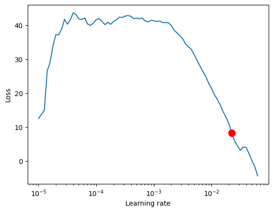
使用PyTorch Lightning找到最佳学习率很容易。
[8]:
# find optimal learning rate
from lightning.pytorch.tuner import Tuner

res = Tuner(trainer).lr_find(
    net,
    train_dataloaders=train_dataloader,
    val_dataloaders=val_dataloader,
    min_lr=1e-5,
    max_lr=1e0,
    early_stop_threshold=100,
)
print(f"suggested learning rate: {res.suggestion()}")
fig = res.plot(show=True, suggest=True)
fig.show()
net.hparams.learning_rate = res.suggestion()
LR finder stopped early after 76 steps due to diverging loss.
Learning rate set to 0.022387211385683406
Restoring states from the checkpoint path at /Users/JanBeitner/Documents/code/pytorch-forecasting/.lr_find_f89a547a-b375-400f-be1c-512fb11fc610.ckpt
Restored all states from the checkpoint at /Users/JanBeitner/Documents/code/pytorch-forecasting/.lr_find_f89a547a-b375-400f-be1c-512fb11fc610.ckpt
suggested learning rate: 0.022387211385683406
[9]:
early_stop_callback = EarlyStopping(monitor="val_loss", min_delta=1e-4, patience=10, verbose=False, mode="min")
trainer = pl.Trainer(
    max_epochs=30,
    accelerator="cpu",
    enable_model_summary=True,
    gradient_clip_val=0.1,
    callbacks=[early_stop_callback],
    limit_train_batches=50,
    enable_checkpointing=True,
)


net = DeepAR.from_dataset(
    training,
    learning_rate=1e-2,
    log_interval=10,
    log_val_interval=1,
    hidden_size=30,
    rnn_layers=2,
    optimizer="Adam",
    loss=MultivariateNormalDistributionLoss(rank=30),
)

trainer.fit(
    net,
    train_dataloaders=train_dataloader,
    val_dataloaders=val_dataloader,
)
GPU available: True (mps), used: False
TPU available: False, using: 0 TPU cores
IPU available: False, using: 0 IPUs
HPU available: False, using: 0 HPUs

  | Name                   | Type                               | Params
------------------------------------------------------------------------------
0 | loss                   | MultivariateNormalDistributionLoss | 0
1 | logging_metrics        | ModuleList                         | 0
2 | embeddings             | MultiEmbedding                     | 2.1 K
3 | rnn                    | LSTM                               | 13.9 K
4 | distribution_projector | Linear                             | 992
------------------------------------------------------------------------------
17.0 K    Trainable params
0         Non-trainable params
17.0 K    Total params
0.068     Total estimated model params size (MB)
`Trainer.fit` stopped: `max_epochs=30` reached.
[10]:
best_model_path = trainer.checkpoint_callback.best_model_path
best_model = DeepAR.load_from_checkpoint(best_model_path)
[11]:
# best_model = net
predictions = best_model.predict(val_dataloader, trainer_kwargs=dict(accelerator="cpu"), return_y=True)
MAE()(predictions.output, predictions.y)
GPU available: True (mps), used: False
TPU available: False, using: 0 TPU cores
IPU available: False, using: 0 IPUs
HPU available: False, using: 0 HPUs
[11]:
tensor(0.2782)
[12]:
raw_predictions = net.predict(
    val_dataloader, mode="raw", return_x=True, n_samples=100, trainer_kwargs=dict(accelerator="cpu")
)
GPU available: True (mps), used: False
TPU available: False, using: 0 TPU cores
IPU available: False, using: 0 IPUs
HPU available: False, using: 0 HPUs
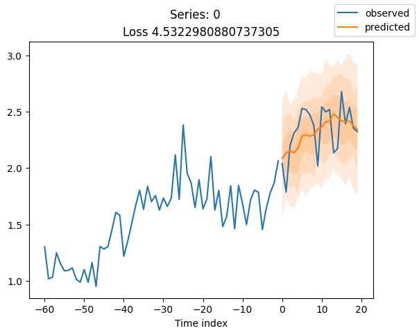
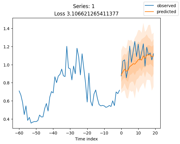
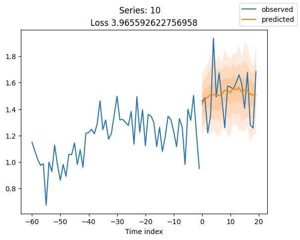
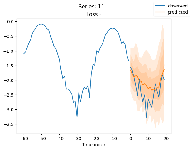
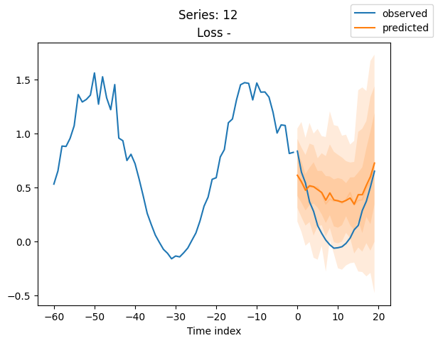
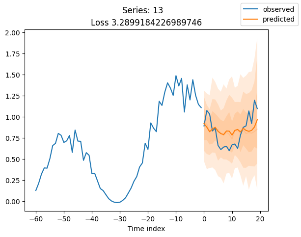
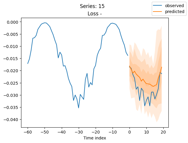
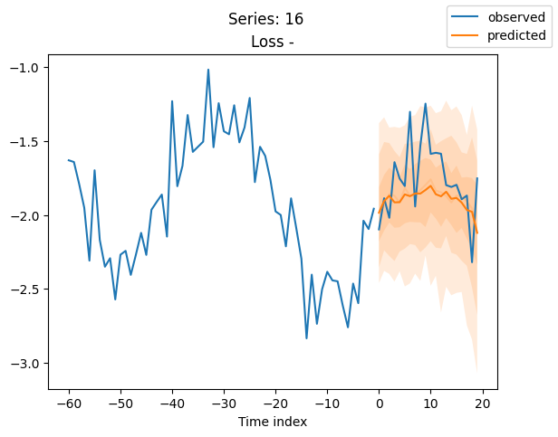
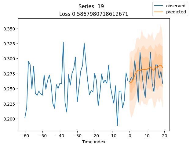
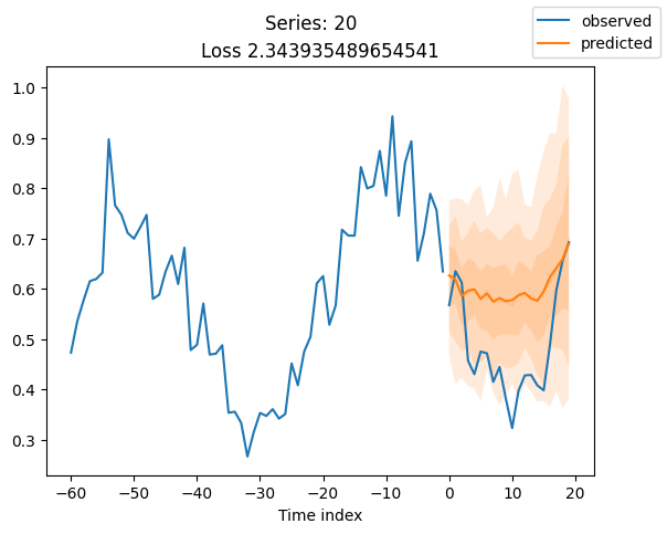
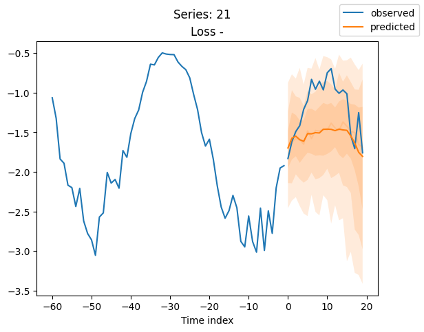
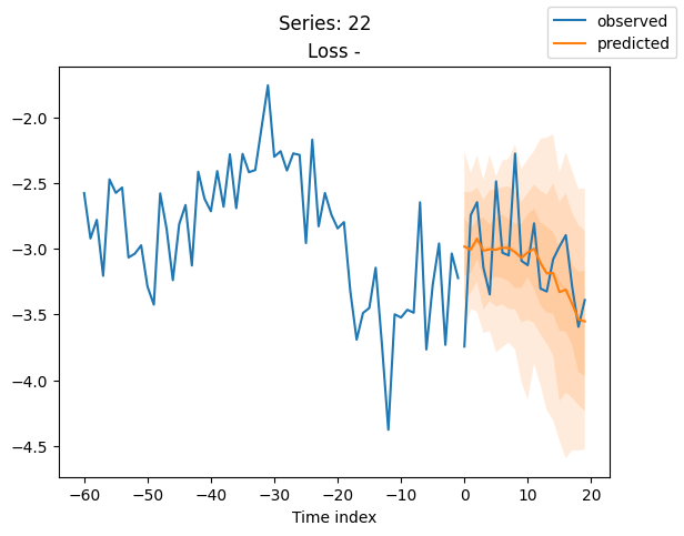
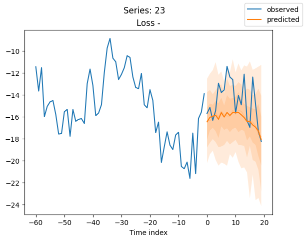
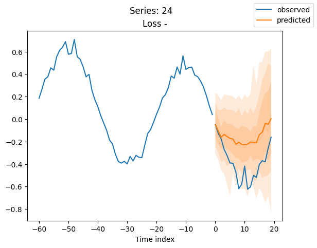
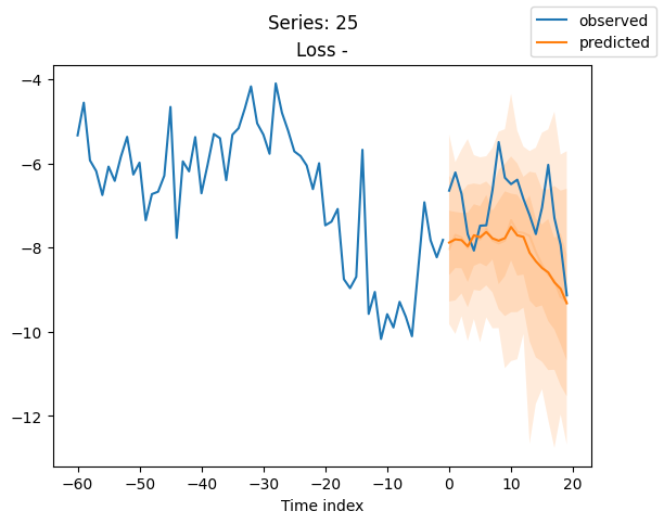
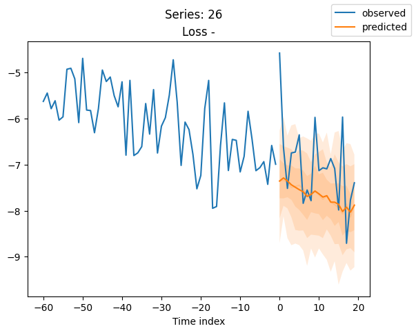
[13]:
series = validation.x_to_index(raw_predictions.x)["series"]
for idx in range(20):  # plot 10 examples
    best_model.plot_prediction(raw_predictions.x, raw_predictions.output, idx=idx, add_loss_to_title=True)
    plt.suptitle(f"Series: {series.iloc[idx]}")


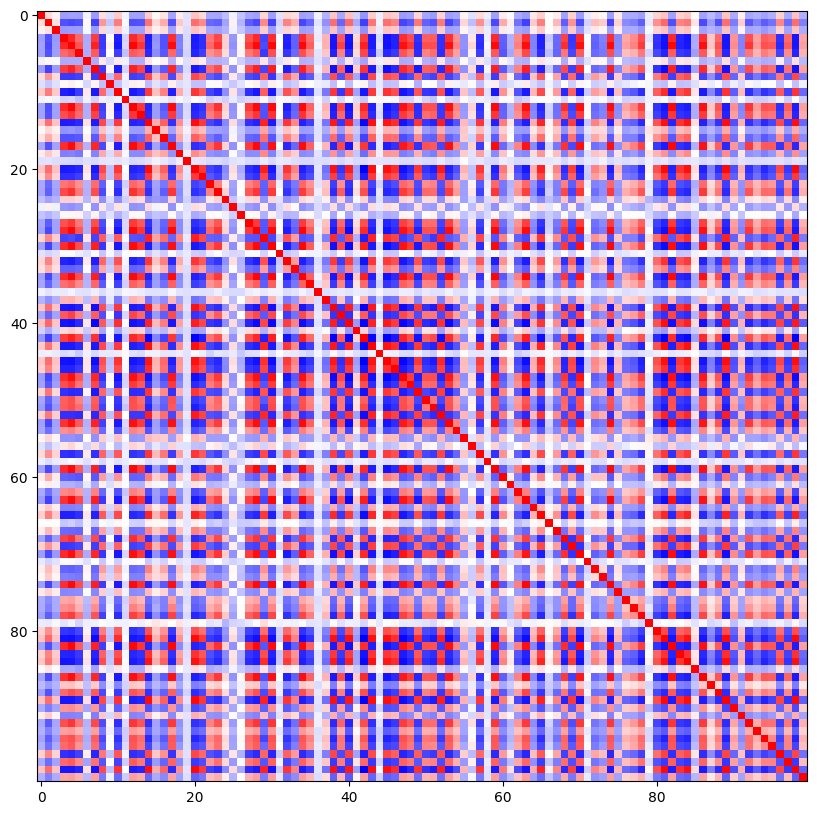
当使用DeepVAR作为多元预测器时,我们可能还对相关矩阵感兴趣。在这里,序列之间没有相关性,我们可能需要更长时间的训练才能显示出这一点。
[14]:
cov_matrix = best_model.loss.map_x_to_distribution(
    best_model.predict(
        val_dataloader, mode=("raw", "prediction"), n_samples=None, trainer_kwargs=dict(accelerator="cpu")
    )
).base_dist.covariance_matrix.mean(0)

# normalize the covariance matrix diagnoal to 1.0
correlation_matrix = cov_matrix / torch.sqrt(torch.diag(cov_matrix)[None] * torch.diag(cov_matrix)[None].T)

fig, ax = plt.subplots(1, 1, figsize=(10, 10))
ax.imshow(correlation_matrix, cmap="bwr")
GPU available: True (mps), used: False
TPU available: False, using: 0 TPU cores
IPU available: False, using: 0 IPUs
HPU available: False, using: 0 HPUs
[14]:
<matplotlib.image.AxesImage at 0x2c4118d90>
[15]:
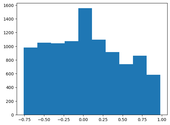
# distribution of off-diagonal correlations
plt.hist(correlation_matrix[correlation_matrix < 1].numpy())
[15]:
(array([ 982., 1052., 1042., 1072., 1554., 1098.,  916.,  738.,  862.,
         584.]),
 array([-0.76116514, -0.58684874, -0.4125323 , -0.23821589, -0.06389947,
         0.11041695,  0.28473336,  0.45904979,  0.63336623,  0.80768263,
         0.98199904]),
 <BarContainer object of 10 artists>)