普通最小二乘法
[1]:
%matplotlib inline
[2]:
import matplotlib.pyplot as plt
import numpy as np
import pandas as pd
import statsmodels.api as sm

np.random.seed(9876789)
OLS 估计
人工数据:
[3]:
nsample = 100
x = np.linspace(0, 10, 100)
X = np.column_stack((x, x ** 2))
beta = np.array([1, 0.1, 10])
e = np.random.normal(size=nsample)
我们的模型需要一个截距,因此我们添加一列1:
[4]:
X = sm.add_constant(X)
y = np.dot(X, beta) + e
拟合和总结:
[5]:
model = sm.OLS(y, X)
results = model.fit()
print(results.summary())
                            OLS Regression Results
==============================================================================
Dep. Variable:                      y   R-squared:                       1.000
Model:                            OLS   Adj. R-squared:                  1.000
Method:                 Least Squares   F-statistic:                 4.020e+06
Date:                Wed, 16 Oct 2024   Prob (F-statistic):          2.83e-239
Time:                        18:27:21   Log-Likelihood:                -146.51
No. Observations:                 100   AIC:                             299.0
Df Residuals:                      97   BIC:                             306.8
Df Model:                           2
Covariance Type:            nonrobust
==============================================================================
                 coef    std err          t      P>|t|      [0.025      0.975]
------------------------------------------------------------------------------
const          1.3423      0.313      4.292      0.000       0.722       1.963
x1            -0.0402      0.145     -0.278      0.781      -0.327       0.247
x2            10.0103      0.014    715.745      0.000       9.982      10.038
==============================================================================
Omnibus:                        2.042   Durbin-Watson:                   2.274
Prob(Omnibus):                  0.360   Jarque-Bera (JB):                1.875
Skew:                           0.234   Prob(JB):                        0.392
Kurtosis:                       2.519   Cond. No.                         144.
==============================================================================

Notes:
[1] Standard Errors assume that the covariance matrix of the errors is correctly specified.
可以直接从拟合模型中提取感兴趣的量。输入 dir(results) 以获取完整列表。以下是一些示例:
[6]:
print("Parameters: ", results.params)
print("R2: ", results.rsquared)
Parameters:  [ 1.34233516 -0.04024948 10.01025357]
R2:  0.9999879365025871
OLS非线性曲线但参数线性
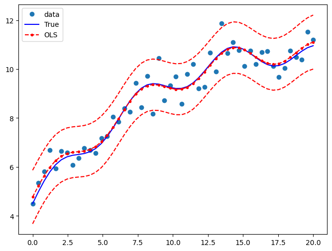
我们模拟了具有x和y之间非线性关系的人工数据:
[7]:
nsample = 50
sig = 0.5
x = np.linspace(0, 20, nsample)
X = np.column_stack((x, np.sin(x), (x - 5) ** 2, np.ones(nsample)))
beta = [0.5, 0.5, -0.02, 5.0]

y_true = np.dot(X, beta)
y = y_true + sig * np.random.normal(size=nsample)
拟合和总结:
[8]:
res = sm.OLS(y, X).fit()
print(res.summary())
                            OLS Regression Results
==============================================================================
Dep. Variable:                      y   R-squared:                       0.933
Model:                            OLS   Adj. R-squared:                  0.928
Method:                 Least Squares   F-statistic:                     211.8
Date:                Wed, 16 Oct 2024   Prob (F-statistic):           6.30e-27
Time:                        18:27:21   Log-Likelihood:                -34.438
No. Observations:                  50   AIC:                             76.88
Df Residuals:                      46   BIC:                             84.52
Df Model:                           3
Covariance Type:            nonrobust
==============================================================================
                 coef    std err          t      P>|t|      [0.025      0.975]
------------------------------------------------------------------------------
x1             0.4687      0.026     17.751      0.000       0.416       0.522
x2             0.4836      0.104      4.659      0.000       0.275       0.693
x3            -0.0174      0.002     -7.507      0.000      -0.022      -0.013
const          5.2058      0.171     30.405      0.000       4.861       5.550
==============================================================================
Omnibus:                        0.655   Durbin-Watson:                   2.896
Prob(Omnibus):                  0.721   Jarque-Bera (JB):                0.360
Skew:                           0.207   Prob(JB):                        0.835
Kurtosis:                       3.026   Cond. No.                         221.
==============================================================================

Notes:
[1] Standard Errors assume that the covariance matrix of the errors is correctly specified.
提取其他感兴趣的量:
[9]:
print("Parameters: ", res.params)
print("Standard errors: ", res.bse)
print("Predicted values: ", res.predict())
Parameters:  [ 0.46872448  0.48360119 -0.01740479  5.20584496]
Standard errors:  [0.02640602 0.10380518 0.00231847 0.17121765]
Predicted values:  [ 4.77072516  5.22213464  5.63620761  5.98658823  6.25643234  6.44117491
  6.54928009  6.60085051  6.62432454  6.6518039   6.71377946  6.83412169
  7.02615877  7.29048685  7.61487206  7.97626054  8.34456611  8.68761335
  8.97642389  9.18997755  9.31866582  9.36587056  9.34740836  9.28893189
  9.22171529  9.17751587  9.1833565   9.25708583  9.40444579  9.61812821
  9.87897556 10.15912843 10.42660281 10.65054491 10.8063004  10.87946503
 10.86825119 10.78378163 10.64826203 10.49133265 10.34519853 10.23933827
 10.19566084 10.22490593 10.32487947 10.48081414 10.66779556 10.85485568
 11.01006072 11.10575781]
绘制一个图表以比较真实关系与OLS预测。预测的置信区间是使用wls_prediction_std命令构建的。
[10]:
pred_ols = res.get_prediction()
iv_l = pred_ols.summary_frame()["obs_ci_lower"]
iv_u = pred_ols.summary_frame()["obs_ci_upper"]

fig, ax = plt.subplots(figsize=(8, 6))

ax.plot(x, y, "o", label="data")
ax.plot(x, y_true, "b-", label="True")
ax.plot(x, res.fittedvalues, "r--.", label="OLS")
ax.plot(x, iv_u, "r--")
ax.plot(x, iv_l, "r--")
ax.legend(loc="best")
[10]:
<matplotlib.legend.Legend at 0x12ad83b10>
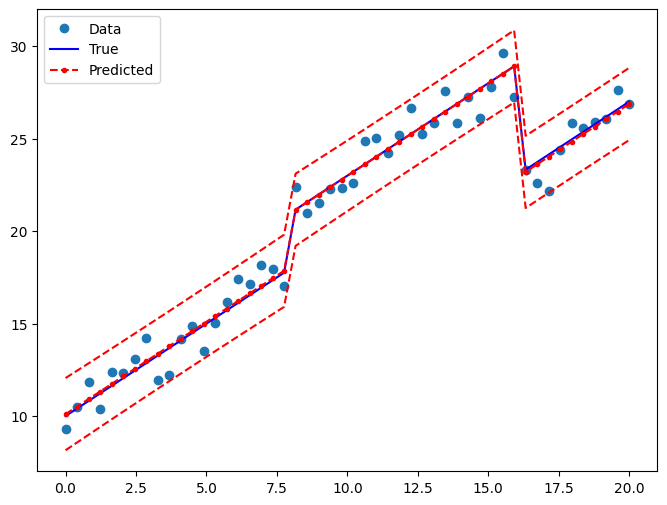
带有虚拟变量的OLS
我们生成了一些人工数据。有3个组将使用虚拟变量进行建模。组0是被省略/基准类别。
[11]:
nsample = 50
groups = np.zeros(nsample, int)
groups[20:40] = 1
groups[40:] = 2
# dummy = (groups[:,None] == np.unique(groups)).astype(float)

dummy = pd.get_dummies(groups).values
x = np.linspace(0, 20, nsample)
# drop reference category
X = np.column_stack((x, dummy[:, 1:]))
X = sm.add_constant(X, prepend=False)

beta = [1.0, 3, -3, 10]
y_true = np.dot(X, beta)
e = np.random.normal(size=nsample)
y = y_true + e
检查数据:
[12]:
print(X[:5, :])
print(y[:5])
print(groups)
print(dummy[:5, :])
[[0.         0.         0.         1.        ]
 [0.40816327 0.         0.         1.        ]
 [0.81632653 0.         0.         1.        ]
 [1.2244898  0.         0.         1.        ]
 [1.63265306 0.         0.         1.        ]]
[ 9.28223335 10.50481865 11.84389206 10.38508408 12.37941998]
[0 0 0 0 0 0 0 0 0 0 0 0 0 0 0 0 0 0 0 0 1 1 1 1 1 1 1 1 1 1 1 1 1 1 1 1 1
 1 1 1 2 2 2 2 2 2 2 2 2 2]
[[ True False False]
 [ True False False]
 [ True False False]
 [ True False False]
 [ True False False]]
拟合和总结:
[13]:
res2 = sm.OLS(y, X).fit()
print(res2.summary())
                            OLS Regression Results
==============================================================================
Dep. Variable:                      y   R-squared:                       0.978
Model:                            OLS   Adj. R-squared:                  0.976
Method:                 Least Squares   F-statistic:                     671.7
Date:                Wed, 16 Oct 2024   Prob (F-statistic):           5.69e-38
Time:                        18:27:22   Log-Likelihood:                -64.643
No. Observations:                  50   AIC:                             137.3
Df Residuals:                      46   BIC:                             144.9
Df Model:                           3
Covariance Type:            nonrobust
==============================================================================
                 coef    std err          t      P>|t|      [0.025      0.975]
------------------------------------------------------------------------------
x1             0.9999      0.060     16.689      0.000       0.879       1.121
x2             2.8909      0.569      5.081      0.000       1.746       4.036
x3            -3.2232      0.927     -3.477      0.001      -5.089      -1.357
const         10.1031      0.310     32.573      0.000       9.479      10.727
==============================================================================
Omnibus:                        2.831   Durbin-Watson:                   1.998
Prob(Omnibus):                  0.243   Jarque-Bera (JB):                1.927
Skew:                          -0.279   Prob(JB):                        0.382
Kurtosis:                       2.217   Cond. No.                         96.3
==============================================================================

Notes:
[1] Standard Errors assume that the covariance matrix of the errors is correctly specified.
绘制一个图表以比较真实关系与OLS预测:
[14]:
pred_ols2 = res2.get_prediction()
iv_l = pred_ols2.summary_frame()["obs_ci_lower"]
iv_u = pred_ols2.summary_frame()["obs_ci_upper"]

fig, ax = plt.subplots(figsize=(8, 6))

ax.plot(x, y, "o", label="Data")
ax.plot(x, y_true, "b-", label="True")
ax.plot(x, res2.fittedvalues, "r--.", label="Predicted")
ax.plot(x, iv_u, "r--")
ax.plot(x, iv_l, "r--")
legend = ax.legend(loc="best")
联合假设检验
F检验
我们想要检验的假设是虚拟变量的两个系数都等于零,即 \(R \times \beta = 0\)。F检验使我们强烈拒绝三个组中常数相同的原假设:
[15]:
R = [[0, 1, 0, 0], [0, 0, 1, 0]]
print(np.array(R))
print(res2.f_test(R))
[[0 1 0 0]
 [0 0 1 0]]
<F test: F=145.49268198027877, p=1.2834419617284415e-20, df_denom=46, df_num=2>
您也可以使用类似公式的语法来检验假设
[16]:
print(res2.f_test("x2 = x3 = 0"))
<F test: F=145.49268198027906, p=1.2834419617283935e-20, df_denom=46, df_num=2>
小组效应
如果我们生成具有较小组效应的人工数据,T检验将无法再拒绝原假设:
[17]:
beta = [1.0, 0.3, -0.0, 10]
y_true = np.dot(X, beta)
y = y_true + np.random.normal(size=nsample)

res3 = sm.OLS(y, X).fit()
[18]:
print(res3.f_test(R))
<F test: F=1.2249111925408274, p=0.30318644106314596, df_denom=46, df_num=2>
[19]:
print(res3.f_test("x2 = x3 = 0"))
<F test: F=1.2249111925408276, p=0.30318644106314596, df_denom=46, df_num=2>
多重共线性
Longley数据集以其高多重共线性而闻名。也就是说,外生预测变量之间高度相关。这是有问题的,因为它可能会在我们对模型规范进行微小更改时影响我们系数估计的稳定性。
[20]:
from statsmodels.datasets.longley import load_pandas

y = load_pandas().endog
X = load_pandas().exog
X = sm.add_constant(X)
拟合和总结:
[21]:
ols_model = sm.OLS(y, X)
ols_results = ols_model.fit()
print(ols_results.summary())
                            OLS Regression Results
==============================================================================
Dep. Variable:                 TOTEMP   R-squared:                       0.995
Model:                            OLS   Adj. R-squared:                  0.992
Method:                 Least Squares   F-statistic:                     330.3
Date:                Wed, 16 Oct 2024   Prob (F-statistic):           4.98e-10
Time:                        18:27:22   Log-Likelihood:                -109.62
No. Observations:                  16   AIC:                             233.2
Df Residuals:                       9   BIC:                             238.6
Df Model:                           6
Covariance Type:            nonrobust
==============================================================================
                 coef    std err          t      P>|t|      [0.025      0.975]
------------------------------------------------------------------------------
const      -3.482e+06    8.9e+05     -3.911      0.004    -5.5e+06   -1.47e+06
GNPDEFL       15.0619     84.915      0.177      0.863    -177.029     207.153
GNP           -0.0358      0.033     -1.070      0.313      -0.112       0.040
UNEMP         -2.0202      0.488     -4.136      0.003      -3.125      -0.915
ARMED         -1.0332      0.214     -4.822      0.001      -1.518      -0.549
POP           -0.0511      0.226     -0.226      0.826      -0.563       0.460
YEAR        1829.1515    455.478      4.016      0.003     798.788    2859.515
==============================================================================
Omnibus:                        0.749   Durbin-Watson:                   2.559
Prob(Omnibus):                  0.688   Jarque-Bera (JB):                0.684
Skew:                           0.420   Prob(JB):                        0.710
Kurtosis:                       2.434   Cond. No.                     4.86e+09
==============================================================================

Notes:
[1] Standard Errors assume that the covariance matrix of the errors is correctly specified.
[2] The condition number is large, 4.86e+09. This might indicate that there are
strong multicollinearity or other numerical problems.
/Users/cw/baidu/code/fin_tool/github/statsmodels/venv/lib/python3.11/site-packages/scipy/stats/_axis_nan_policy.py:418: UserWarning: `kurtosistest` p-value may be inaccurate with fewer than 20 observations; only n=16 observations were given.
  return hypotest_fun_in(*args, **kwds)
条件数
评估多重共线性的一种方法是计算条件数。超过20的值令人担忧(参见Greene 4.9)。第一步是将自变量归一化,使其具有单位长度:
[22]:
norm_x = X.values
for i, name in enumerate(X):
    if name == "const":
        continue
    norm_x[:, i] = X[name] / np.linalg.norm(X[name])
norm_xtx = np.dot(norm_x.T, norm_x)
然后,我们取最大特征值与最小特征值之比的平方根。
[23]:
eigs = np.linalg.eigvals(norm_xtx)
condition_number = np.sqrt(eigs.max() / eigs.min())
print(condition_number)
56240.87047266957
删除一个观察值
格林还指出,删除单个观测值可能会对系数估计产生显著影响:
[24]:
ols_results2 = sm.OLS(y.iloc[:14], X.iloc[:14]).fit()
print(
    "Percentage change %4.2f%%\n"
    * 7
    % tuple(
        [
            i
            for i in (ols_results2.params - ols_results.params)
            / ols_results.params
            * 100
        ]
    )
)
Percentage change 4.55%
Percentage change -105.20%
Percentage change -3.43%
Percentage change 2.92%
Percentage change 3.32%
Percentage change 97.06%
Percentage change 4.64%
我们也可以查看这方面的正式统计数据,例如DFBETAS – 这是一个标准化的度量,用于衡量当排除该观测值时,每个系数的变化程度。
[25]:
infl = ols_results.get_influence()
一般来说,我们可以认为绝对值大于 \(2/\sqrt{N}\) 的 DBETAS 是有影响力的观测值
[26]:
2.0 / len(X) ** 0.5
[26]:
0.5
[27]:
print(infl.summary_frame().filter(regex="dfb"))
    dfb_const  dfb_GNPDEFL   dfb_GNP  dfb_UNEMP  dfb_ARMED   dfb_POP  dfb_YEAR
0   -0.016406    -0.234566 -0.045095  -0.121513  -0.149026  0.211057  0.013388
1   -0.020608    -0.289091  0.124453   0.156964   0.287700 -0.161890  0.025958
2   -0.008382     0.007161 -0.016799   0.009575   0.002227  0.014871  0.008103
3    0.018093     0.907968 -0.500022  -0.495996   0.089996  0.711142 -0.040056
4    1.871260    -0.219351  1.611418   1.561520   1.169337 -1.081513 -1.864186
5   -0.321373    -0.077045 -0.198129  -0.192961  -0.430626  0.079916  0.323275
6    0.315945    -0.241983  0.438146   0.471797  -0.019546 -0.448515 -0.307517
7    0.015816    -0.002742  0.018591   0.005064  -0.031320 -0.015823 -0.015583
8   -0.004019    -0.045687  0.023708   0.018125   0.013683 -0.034770  0.005116
9   -1.018242    -0.282131 -0.412621  -0.663904  -0.715020 -0.229501  1.035723
10   0.030947    -0.024781  0.029480   0.035361   0.034508 -0.014194 -0.030805
11   0.005987    -0.079727  0.030276  -0.008883  -0.006854 -0.010693 -0.005323
12  -0.135883     0.092325 -0.253027  -0.211465   0.094720  0.331351  0.129120
13   0.032736    -0.024249  0.017510   0.033242   0.090655  0.007634 -0.033114
14   0.305868     0.148070  0.001428   0.169314   0.253431  0.342982 -0.318031
15  -0.538323     0.432004 -0.261262  -0.143444  -0.360890 -0.467296  0.552421
Last update:
Oct 16, 2024