回归诊断
这个示例文件展示了如何在实际生活中使用一些statsmodels回归诊断测试。你可以在回归诊断页面上了解更多测试并获取更多信息。
请注意,这里描述的大多数测试只返回一个数字元组,没有任何注释。输出的完整描述总是包含在docstring和在线的statsmodels文档中。为了演示目的,我们在下面的示例中使用zip(name,test)构造来美观地打印简短描述。
估计一个回归模型
[1]:
%matplotlib inline
[2]:
from statsmodels.compat import lzip

import numpy as np
import pandas as pd
import statsmodels.formula.api as smf
import statsmodels.stats.api as sms
import matplotlib.pyplot as plt

# Load data
url = "https://raw.githubusercontent.com/vincentarelbundock/Rdatasets/master/csv/HistData/Guerry.csv"
dat = pd.read_csv(url)

# Fit regression model (using the natural log of one of the regressors)
results = smf.ols("Lottery ~ Literacy + np.log(Pop1831)", data=dat).fit()

# Inspect the results
print(results.summary())
                            OLS Regression Results
==============================================================================
Dep. Variable:                Lottery   R-squared:                       0.348
Model:                            OLS   Adj. R-squared:                  0.333
Method:                 Least Squares   F-statistic:                     22.20
Date:                Wed, 16 Oct 2024   Prob (F-statistic):           1.90e-08
Time:                        18:27:14   Log-Likelihood:                -379.82
No. Observations:                  86   AIC:                             765.6
Df Residuals:                      83   BIC:                             773.0
Df Model:                           2
Covariance Type:            nonrobust
===================================================================================
                      coef    std err          t      P>|t|      [0.025      0.975]
-----------------------------------------------------------------------------------
Intercept         246.4341     35.233      6.995      0.000     176.358     316.510
Literacy           -0.4889      0.128     -3.832      0.000      -0.743      -0.235
np.log(Pop1831)   -31.3114      5.977     -5.239      0.000     -43.199     -19.424
==============================================================================
Omnibus:                        3.713   Durbin-Watson:                   2.019
Prob(Omnibus):                  0.156   Jarque-Bera (JB):                3.394
Skew:                          -0.487   Prob(JB):                        0.183
Kurtosis:                       3.003   Cond. No.                         702.
==============================================================================

Notes:
[1] Standard Errors assume that the covariance matrix of the errors is correctly specified.
残差的正态性
Jarque-Bera 检验:
[3]:
name = ["Jarque-Bera", "Chi^2 two-tail prob.", "Skew", "Kurtosis"]
test = sms.jarque_bera(results.resid)
lzip(name, test)
[3]:
[('Jarque-Bera', np.float64(3.3936080248431657)),
 ('Chi^2 two-tail prob.', np.float64(0.1832683123166338)),
 ('Skew', np.float64(-0.4865803431122337)),
 ('Kurtosis', np.float64(3.0034177578816323))]
全渠道测试:
[4]:
name = ["Chi^2", "Two-tail probability"]
test = sms.omni_normtest(results.resid)
lzip(name, test)
[4]:
[('Chi^2', np.float64(3.71343781159718)),
 ('Two-tail probability', np.float64(0.15618424580304832))]
影响测试
一旦创建,类 OLSInfluence 的对象会保存属性和方法,允许用户评估每个观测值的影响。例如,我们可以通过以下方式计算并提取 DFbetas 的前几行:
[5]:
from statsmodels.stats.outliers_influence import OLSInfluence

test_class = OLSInfluence(results)
test_class.dfbetas[:5, :]
[5]:
array([[-0.00301154,  0.00290872,  0.00118179],
       [-0.06425662,  0.04043093,  0.06281609],
       [ 0.01554894, -0.03556038, -0.00905336],
       [ 0.17899858,  0.04098207, -0.18062352],
       [ 0.29679073,  0.21249207, -0.3213655 ]])
通过输入 dir(influence_test) 探索其他选项
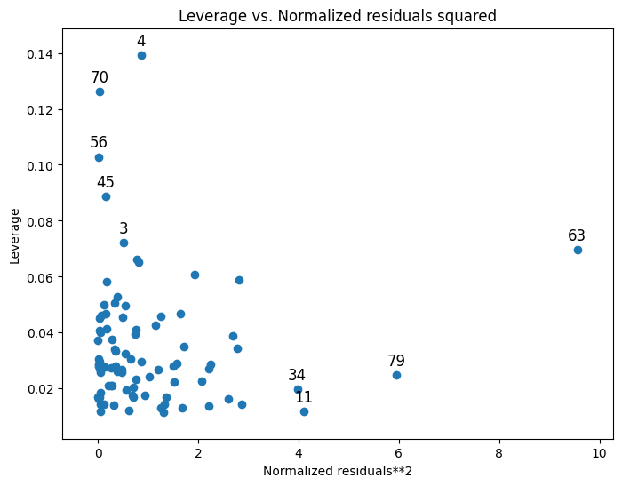
关于杠杆的有用信息也可以绘制:
[6]:
from statsmodels.graphics.regressionplots import plot_leverage_resid2

fig, ax = plt.subplots(figsize=(8, 6))
fig = plot_leverage_resid2(results, ax=ax)
其他绘图选项可以在图形页面上找到。
多重共线性
条件数:
[7]:
np.linalg.cond(results.model.exog)
[7]:
np.float64(702.1792145490065)
异方差性检验
Breush-Pagan 检验:
[8]:
name = ["Lagrange multiplier statistic", "p-value", "f-value", "f p-value"]
test = sms.het_breuschpagan(results.resid, results.model.exog)
lzip(name, test)
[8]:
[('Lagrange multiplier statistic', np.float64(4.893213374093985)),
 ('p-value', np.float64(0.08658690502352087)),
 ('f-value', np.float64(2.503715946256453)),
 ('f p-value', np.float64(0.08794028782672857))]
Goldfeld-Quandt 检验
[9]:
name = ["F statistic", "p-value"]
test = sms.het_goldfeldquandt(results.resid, results.model.exog)
lzip(name, test)
[9]:
[('F statistic', np.float64(1.1002422436378152)),
 ('p-value', np.float64(0.3820295068692518))]
线性
Harvey-Collier 乘数检验,用于检验线性规范正确的零假设:
[10]:
name = ["t value", "p value"]
test = sms.linear_harvey_collier(results)
lzip(name, test)
[10]:
[('t value', np.float64(-1.0796490077784027)),
 ('p value', np.float64(0.2834639247558495))]
Last update:
Oct 16, 2024