递归最小二乘法
递归最小二乘法是普通最小二乘法的一个扩展窗口版本。除了递归计算的回归系数外,递归计算的残差还可以用于构建统计量来研究参数的不稳定性。
类RecursiveLS允许计算递归残差并计算CUSUM和CUSUM平方统计量。绘制这些统计量以及表示参数稳定性的零假设下统计显著偏差的参考线,可以轻松直观地指示参数稳定性。
最后,RecursiveLS 模型允许对参数向量施加线性限制,并且可以使用公式接口进行构建。
[1]:
%matplotlib inline
import matplotlib.pyplot as plt
import numpy as np
import pandas as pd
import statsmodels.api as sm
from pandas_datareader.data import DataReader

np.set_printoptions(suppress=True)
示例 1: 铜
我们首先考虑铜数据集中的参数稳定性(描述如下)。
[2]:
print(sm.datasets.copper.DESCRLONG)

dta = sm.datasets.copper.load_pandas().data
dta.index = pd.date_range("1951-01-01", "1975-01-01", freq="YS")
endog = dta["WORLDCONSUMPTION"]

# To the regressors in the dataset, we add a column of ones for an intercept
exog = sm.add_constant(
    dta[["COPPERPRICE", "INCOMEINDEX", "ALUMPRICE", "INVENTORYINDEX"]]
)
This data describes the world copper market from 1951 through 1975.  In an
example, in Gill, the outcome variable (of a 2 stage estimation) is the world
consumption of copper for the 25 years.  The explanatory variables are the
world consumption of copper in 1000 metric tons, the constant dollar adjusted
price of copper, the price of a substitute, aluminum, an index of real per
capita income base 1970, an annual measure of manufacturer inventory change,
and a time trend.
首先,构建并拟合模型,并打印摘要。尽管RLS模型递归地计算回归参数,因此每个数据点都有一个估计值,但摘要表仅显示在整个样本上估计的回归参数;除了递归初始化带来的微小影响外,这些估计值与OLS估计值是等价的。
[3]:
mod = sm.RecursiveLS(endog, exog)
res = mod.fit()

print(res.summary())
                           Statespace Model Results
==============================================================================
Dep. Variable:       WORLDCONSUMPTION   No. Observations:                   25
Model:                    RecursiveLS   Log Likelihood                -154.720
Date:                Wed, 16 Oct 2024   R-squared:                       0.965
Time:                        18:27:43   AIC                            319.441
Sample:                    01-01-1951   BIC                            325.535
                         - 01-01-1975   HQIC                           321.131
Covariance Type:            nonrobust   Scale                       117717.127
==================================================================================
                     coef    std err          z      P>|z|      [0.025      0.975]
----------------------------------------------------------------------------------
const          -6562.3719   2378.939     -2.759      0.006   -1.12e+04   -1899.737
COPPERPRICE      -13.8132     15.041     -0.918      0.358     -43.292      15.666
INCOMEINDEX      1.21e+04    763.401     15.853      0.000    1.06e+04    1.36e+04
ALUMPRICE         70.4146     32.678      2.155      0.031       6.367     134.462
INVENTORYINDEX   311.7330   2130.084      0.146      0.884   -3863.155    4486.621
===================================================================================
Ljung-Box (L1) (Q):                   2.17   Jarque-Bera (JB):                 1.70
Prob(Q):                              0.14   Prob(JB):                         0.43
Heteroskedasticity (H):               3.38   Skew:                            -0.67
Prob(H) (two-sided):                  0.13   Kurtosis:                         2.53
===================================================================================

Warnings:
[1] Parameters and covariance matrix estimates are RLS estimates conditional on the entire sample.
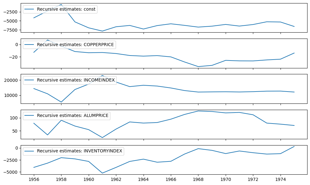
递归系数可以在 recursive_coefficients 属性中找到。或者,可以使用 plot_recursive_coefficient 方法生成图表。
[4]:
print(res.recursive_coefficients.filtered[0])
res.plot_recursive_coefficient(range(mod.k_exog), alpha=None, figsize=(10, 6))
[     2.88890087      4.94795049   1558.41803044   1958.43326657
 -51474.95496072  -4168.95103556  -2252.61354153   -446.55912855
  -5288.39795381  -6942.31935664  -7846.08903015  -6643.1512165
  -6274.11015898  -7272.01696641  -6319.02648863  -5822.23929403
  -6256.30902929  -6737.40446161  -6477.42841703  -5995.90747251
  -6450.80678164  -6022.92166726  -5258.35152757  -5320.89136355
  -6562.3719344 ]
[4]:

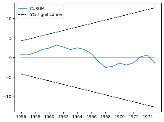
CUSUM统计量可以在cusum属性中找到,但通常使用plot_cusum方法进行参数稳定性的视觉检查更为方便。在下图中,CUSUM统计量没有超出5%显著性区间,因此我们无法在5%的水平上拒绝参数稳定的原假设。
[5]:
print(res.cusum)
fig = res.plot_cusum()
[ 0.69971507  0.6584124   1.24629671  2.05476028  2.39888915  3.17861977
  2.67244669  2.01783212  2.46131744  2.05268635  0.95054333 -1.0450555
 -2.55465289 -2.29908155 -1.45289496 -1.95353997 -1.35046624  0.15789825
  0.63286527 -1.48184589]
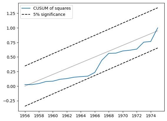
另一个相关的统计量是平方和的CUSUM。它可以在cusum_squares属性中找到,但同样更方便的是通过plot_cusum_squares方法进行可视化检查。在下图中,平方和的CUSUM统计量没有超出5%显著性区间,因此我们未能以5%的显著性水平拒绝参数稳定的原假设。
[6]:
res.plot_cusum_squares()
[6]:

示例 2: 货币数量理论
货币数量理论表明,“货币数量变化率的给定变化会引发……价格通胀率相等的变化”(Lucas,1980)。根据Lucas的研究,我们考察了货币增长的双边指数加权移动平均与CPI通胀之间的关系。尽管Lucas发现这些变量之间的关系是稳定的,但最近的研究表明这种关系是不稳定的;参见例如Sargent和Surico(2010)。
[7]:
start = "1959-12-01"
end = "2015-01-01"
m2 = DataReader("M2SL", "fred", start=start, end=end)
cpi = DataReader("CPIAUCSL", "fred", start=start, end=end)
[8]:
def ewma(series, beta, n_window):
    nobs = len(series)
    scalar = (1 - beta) / (1 + beta)
    ma = []
    k = np.arange(n_window, 0, -1)
    weights = np.r_[beta ** k, 1, beta ** k[::-1]]
    for t in range(n_window, nobs - n_window):
        window = series.iloc[t - n_window : t + n_window + 1].values
        ma.append(scalar * np.sum(weights * window))
    return pd.Series(ma, name=series.name, index=series.iloc[n_window:-n_window].index)


m2_ewma = ewma(np.log(m2["M2SL"].resample("QS").mean()).diff().iloc[1:], 0.95, 10 * 4)
cpi_ewma = ewma(
    np.log(cpi["CPIAUCSL"].resample("QS").mean()).diff().iloc[1:], 0.95, 10 * 4
)
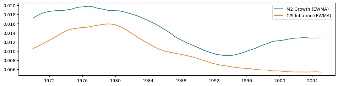
在使用Lucas的\(\beta = 0.95\)滤波器(两边各有10年的窗口)构建移动平均线后,我们在下面绘制了每个序列。尽管它们在前一部分样本中似乎一起移动,但在1990年后它们似乎开始分化。
[9]:
fig, ax = plt.subplots(figsize=(13, 3))

ax.plot(m2_ewma, label="M2 Growth (EWMA)")
ax.plot(cpi_ewma, label="CPI Inflation (EWMA)")
ax.legend()
[9]:
<matplotlib.legend.Legend at 0x1340281d0>
[10]:
endog = cpi_ewma
exog = sm.add_constant(m2_ewma)
exog.columns = ["const", "M2"]

mod = sm.RecursiveLS(endog, exog)
res = mod.fit()

print(res.summary())
                           Statespace Model Results
==============================================================================
Dep. Variable:               CPIAUCSL   No. Observations:                  141
Model:                    RecursiveLS   Log Likelihood                 692.878
Date:                Wed, 16 Oct 2024   R-squared:                       0.813
Time:                        18:27:46   AIC                          -1381.755
Sample:                    01-01-1970   BIC                          -1375.858
                         - 01-01-2005   HQIC                         -1379.358
Covariance Type:            nonrobust   Scale                            0.000
==============================================================================
                 coef    std err          z      P>|z|      [0.025      0.975]
------------------------------------------------------------------------------
const         -0.0034      0.001     -6.013      0.000      -0.004      -0.002
M2             0.9128      0.037     24.601      0.000       0.840       0.986
===================================================================================
Ljung-Box (L1) (Q):                 138.23   Jarque-Bera (JB):                18.20
Prob(Q):                              0.00   Prob(JB):                         0.00
Heteroskedasticity (H):               5.30   Skew:                            -0.81
Prob(H) (two-sided):                  0.00   Kurtosis:                         2.27
===================================================================================

Warnings:
[1] Parameters and covariance matrix estimates are RLS estimates conditional on the entire sample.
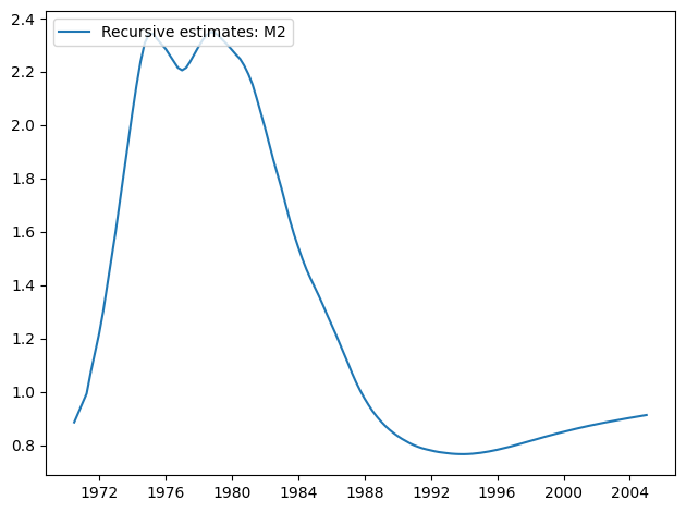
[11]:
res.plot_recursive_coefficient(1, alpha=None)
[11]:

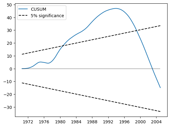
CUSUM 图现在显示在 5% 水平上有显著偏差,表明拒绝参数稳定性原假设。
[12]:
res.plot_cusum()
[12]:

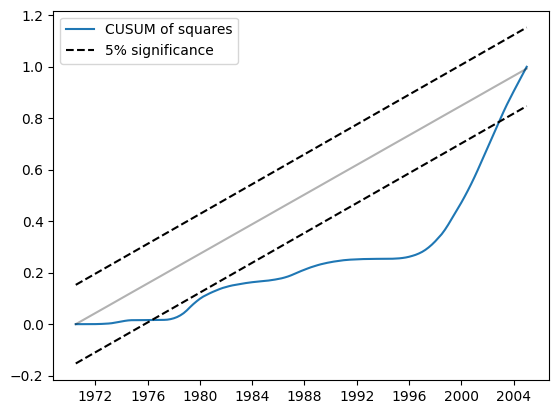
同样地,平方的CUSUM在5%水平上显示出显著的偏差,这也表明拒绝参数稳定性原假设。
[13]:
res.plot_cusum_squares()
[13]:

示例 3: 线性限制和公式
线性限制
使用模型构造中的constraints参数来实现线性限制并不困难。
[14]:
endog = dta["WORLDCONSUMPTION"]
exog = sm.add_constant(
    dta[["COPPERPRICE", "INCOMEINDEX", "ALUMPRICE", "INVENTORYINDEX"]]
)

mod = sm.RecursiveLS(endog, exog, constraints="COPPERPRICE = ALUMPRICE")
res = mod.fit()
print(res.summary())
                           Statespace Model Results
==============================================================================
Dep. Variable:       WORLDCONSUMPTION   No. Observations:                   25
Model:                    RecursiveLS   Log Likelihood                -143.684
Date:                Wed, 16 Oct 2024   R-squared:                       0.989
Time:                        18:27:48   AIC                            295.368
Sample:                    01-01-1951   BIC                            300.244
                         - 01-01-1975   HQIC                           296.721
Covariance Type:            nonrobust   Scale                       137155.014
==================================================================================
                     coef    std err          z      P>|z|      [0.025      0.975]
----------------------------------------------------------------------------------
const          -4839.4893   2412.410     -2.006      0.045   -9567.726    -111.253
COPPERPRICE        5.9797     12.704      0.471      0.638     -18.921      30.880
INCOMEINDEX     1.115e+04    666.308     16.738      0.000    9847.002    1.25e+04
ALUMPRICE          5.9797     12.704      0.471      0.638     -18.921      30.880
INVENTORYINDEX   241.3447   2298.951      0.105      0.916   -4264.516    4747.205
===================================================================================
Ljung-Box (L1) (Q):                   6.27   Jarque-Bera (JB):                 1.78
Prob(Q):                              0.01   Prob(JB):                         0.41
Heteroskedasticity (H):               1.75   Skew:                            -0.63
Prob(H) (two-sided):                  0.48   Kurtosis:                         2.32
===================================================================================

Warnings:
[1] Parameters and covariance matrix estimates are RLS estimates conditional on the entire sample.
[2] Covariance matrix is singular or near-singular, with condition number 3.62e+18. Standard errors may be unstable.
公式
可以使用类方法 from_formula 来拟合同一个模型。
[15]:
mod = sm.RecursiveLS.from_formula(
    "WORLDCONSUMPTION ~ COPPERPRICE + INCOMEINDEX + ALUMPRICE + INVENTORYINDEX",
    dta,
    constraints="COPPERPRICE = ALUMPRICE",
)
res = mod.fit()
print(res.summary())
                           Statespace Model Results
==============================================================================
Dep. Variable:       WORLDCONSUMPTION   No. Observations:                   25
Model:                    RecursiveLS   Log Likelihood                -143.684
Date:                Wed, 16 Oct 2024   R-squared:                       0.989
Time:                        18:27:48   AIC                            295.368
Sample:                    01-01-1951   BIC                            300.244
                         - 01-01-1975   HQIC                           296.721
Covariance Type:            nonrobust   Scale                       137155.014
==================================================================================
                     coef    std err          z      P>|z|      [0.025      0.975]
----------------------------------------------------------------------------------
Intercept      -4839.4893   2412.410     -2.006      0.045   -9567.726    -111.253
COPPERPRICE        5.9797     12.704      0.471      0.638     -18.921      30.880
INCOMEINDEX     1.115e+04    666.308     16.738      0.000    9847.002    1.25e+04
ALUMPRICE          5.9797     12.704      0.471      0.638     -18.921      30.880
INVENTORYINDEX   241.3447   2298.951      0.105      0.916   -4264.516    4747.205
===================================================================================
Ljung-Box (L1) (Q):                   6.27   Jarque-Bera (JB):                 1.78
Prob(Q):                              0.01   Prob(JB):                         0.41
Heteroskedasticity (H):               1.75   Skew:                            -0.63
Prob(H) (two-sided):                  0.48   Kurtosis:                         2.32
===================================================================================

Warnings:
[1] Parameters and covariance matrix estimates are RLS estimates conditional on the entire sample.
[2] Covariance matrix is singular or near-singular, with condition number 3.62e+18. Standard errors may be unstable.
/Users/cw/baidu/code/fin_tool/github/statsmodels/venv/lib/python3.11/site-packages/statsmodels/tsa/base/tsa_model.py:473: ValueWarning: No frequency information was provided, so inferred frequency YS-JAN will be used.
  self._init_dates(dates, freq)