预测(样本外)
[1]:
%matplotlib inline
[2]:
import numpy as np
import matplotlib.pyplot as plt

import statsmodels.api as sm

plt.rc("figure", figsize=(16, 8))
plt.rc("font", size=14)
人工数据
[3]:
nsample = 50
sig = 0.25
x1 = np.linspace(0, 20, nsample)
X = np.column_stack((x1, np.sin(x1), (x1 - 5) ** 2))
X = sm.add_constant(X)
beta = [5.0, 0.5, 0.5, -0.02]
y_true = np.dot(X, beta)
y = y_true + sig * np.random.normal(size=nsample)
估计
[4]:
olsmod = sm.OLS(y, X)
olsres = olsmod.fit()
print(olsres.summary())
                            OLS Regression Results
==============================================================================
Dep. Variable:                      y   R-squared:                       0.979
Model:                            OLS   Adj. R-squared:                  0.978
Method:                 Least Squares   F-statistic:                     722.1
Date:                Wed, 16 Oct 2024   Prob (F-statistic):           1.12e-38
Time:                        18:26:48   Log-Likelihood:                -5.8456
No. Observations:                  50   AIC:                             19.69
Df Residuals:                      46   BIC:                             27.34
Df Model:                           3
Covariance Type:            nonrobust
==============================================================================
                 coef    std err          t      P>|t|      [0.025      0.975]
------------------------------------------------------------------------------
const          4.9642      0.097     51.363      0.000       4.770       5.159
x1             0.5041      0.015     33.822      0.000       0.474       0.534
x2             0.4873      0.059      8.317      0.000       0.369       0.605
x3            -0.0200      0.001    -15.284      0.000      -0.023      -0.017
==============================================================================
Omnibus:                        0.637   Durbin-Watson:                   2.013
Prob(Omnibus):                  0.727   Jarque-Bera (JB):                0.406
Skew:                          -0.220   Prob(JB):                        0.816
Kurtosis:                       2.974   Cond. No.                         221.
==============================================================================

Notes:
[1] Standard Errors assume that the covariance matrix of the errors is correctly specified.
样本内预测
[5]:
ypred = olsres.predict(X)
print(ypred)
[ 4.46416116  4.94167162  5.38073736  5.7547997   6.04688486  6.25239266
  6.3798524   6.44952142  6.49005694  6.53380775  6.61149939  6.74718602
  6.9542984   7.23343726  7.57227459  7.94757911  8.32903309  8.68421347
  8.98391888  9.20696736  9.34367646  9.39745406  9.38423847  9.3298798
  9.26589286  9.22427938  9.2322702   9.30785131  9.45680886  9.67177842
  9.93345503 10.21376487 10.48047778 10.70250251 10.854995   10.92344014
 10.90603655 10.81399261 10.66968487 10.50298171 10.34633603 10.22945329
 10.17441108 10.19203172 10.28010429 10.4237478  10.59785613 10.7712229
 10.91166856 10.99132744]
创建一个新的解释变量样本Xnew,预测并绘图
[6]:
x1n = np.linspace(20.5, 25, 10)
Xnew = np.column_stack((x1n, np.sin(x1n), (x1n - 5) ** 2))
Xnew = sm.add_constant(Xnew)
ynewpred = olsres.predict(Xnew)  # predict out of sample
print(ynewpred)
[10.97923871 10.83821339 10.58736242 10.27023729  9.94416706  9.66622222
  9.47924186  9.40134515  9.42149513  9.50220096]
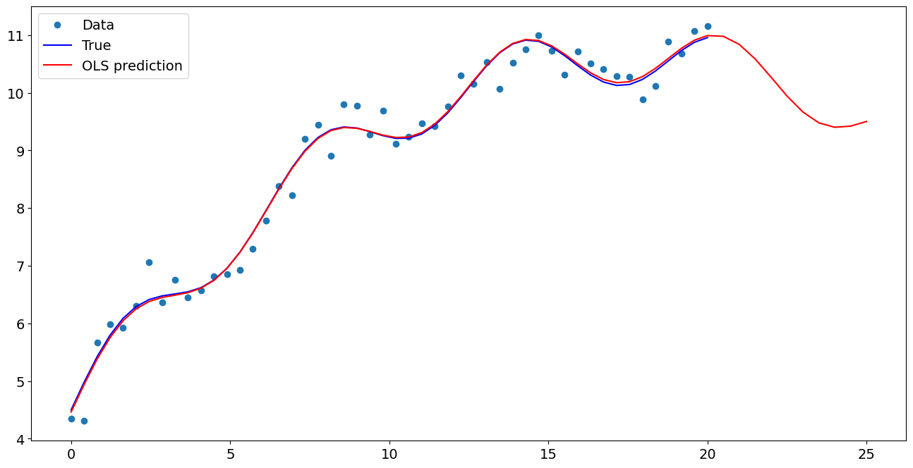
绘图比较
[7]:
import matplotlib.pyplot as plt

fig, ax = plt.subplots()
ax.plot(x1, y, "o", label="Data")
ax.plot(x1, y_true, "b-", label="True")
ax.plot(np.hstack((x1, x1n)), np.hstack((ypred, ynewpred)), "r", label="OLS prediction")
ax.legend(loc="best")
[7]:
<matplotlib.legend.Legend at 0x121851e10>
使用公式进行预测
使用公式可以使估计和预测变得更加容易
[8]:
from statsmodels.formula.api import ols

data = {"x1": x1, "y": y}

res = ols("y ~ x1 + np.sin(x1) + I((x1-5)**2)", data=data).fit()
我们使用I来表示使用身份变换。即,我们不希望在使用**2时产生任何扩展魔法。
[9]:
res.params
[9]:
Intercept           4.964220
x1                  0.504137
np.sin(x1)          0.487323
I((x1 - 5) ** 2)   -0.020002
dtype: float64
现在我们只需要传递单个变量,就可以自动获得转换后的右侧变量
[10]:
res.predict(exog=dict(x1=x1n))
[10]:
0    10.979239
1    10.838213
2    10.587362
3    10.270237
4     9.944167
5     9.666222
6     9.479242
7     9.401345
8     9.421495
9     9.502201
dtype: float64
Last update:
Oct 16, 2024