statsmodels中的预测
本笔记本描述了在 statsmodels 中使用时间序列模型进行预测。
注意:本笔记本仅适用于状态空间模型类,这些类包括:
sm.tsa.SARIMAXsm.tsa.UnobservedComponentssm.tsa.VARMAXsm.tsa.DynamicFactor
[1]:
%matplotlib inline

import numpy as np
import pandas as pd
import statsmodels.api as sm
import matplotlib.pyplot as plt

macrodata = sm.datasets.macrodata.load_pandas().data
macrodata.index = pd.period_range('1959Q1', '2009Q3', freq='Q')
基本示例
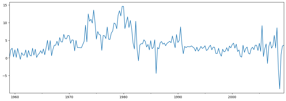
一个简单的例子是使用AR(1)模型来预测通货膨胀。在预测之前,我们先来看一下序列:
[2]:
endog = macrodata['infl']
endog.plot(figsize=(15, 5))
[2]:
<Axes: >
构建和估计模型
下一步是制定我们用于预测的计量经济学模型。在这种情况下,我们将通过 statsmodels 中的 SARIMAX 类使用 AR(1) 模型。
构建模型后,我们需要估计其参数。这是通过使用fit方法完成的。summary方法生成几个方便的表格,显示结果。
[3]:
# Construct the model
mod = sm.tsa.SARIMAX(endog, order=(1, 0, 0), trend='c')
# Estimate the parameters
res = mod.fit()

print(res.summary())
RUNNING THE L-BFGS-B CODE

           * * *

Machine precision = 2.220D-16
 N =            3     M =           10

At X0         0 variables are exactly at the bounds

At iterate    0    f=  2.32873D+00    |proj g|=  8.23649D-03
                               SARIMAX Results
==============================================================================
Dep. Variable:                   infl   No. Observations:                  203
Model:               SARIMAX(1, 0, 0)   Log Likelihood                -472.714
Date:                Wed, 16 Oct 2024   AIC                            951.427
Time:                        18:27:52   BIC                            961.367
Sample:                    03-31-1959   HQIC                           955.449
                         - 09-30-2009
Covariance Type:                  opg
==============================================================================
                 coef    std err          z      P>|z|      [0.025      0.975]
------------------------------------------------------------------------------
intercept      1.3962      0.254      5.488      0.000       0.898       1.895
ar.L1          0.6441      0.039     16.482      0.000       0.568       0.721
sigma2         6.1519      0.397     15.487      0.000       5.373       6.930
===================================================================================
Ljung-Box (L1) (Q):                   8.43   Jarque-Bera (JB):                68.45
Prob(Q):                              0.00   Prob(JB):                         0.00
Heteroskedasticity (H):               1.47   Skew:                            -0.22
Prob(H) (two-sided):                  0.12   Kurtosis:                         5.81
===================================================================================

Warnings:
[1] Covariance matrix calculated using the outer product of gradients (complex-step).
This problem is unconstrained.
预测
使用结果对象中的 forecast 或 get_forecast 方法生成样本外预测。
The forecast 方法仅提供点预测。
[4]:
# The default is to get a one-step-ahead forecast:
print(res.forecast())
2009Q4    3.68921
Freq: Q-DEC, dtype: float64
The get_forecast 方法更通用,并且还可以构建置信区间。
[5]:
# Here we construct a more complete results object.
fcast_res1 = res.get_forecast()

# Most results are collected in the `summary_frame` attribute.
# Here we specify that we want a confidence level of 90%
print(fcast_res1.summary_frame(alpha=0.10))
infl       mean   mean_se  mean_ci_lower  mean_ci_upper
2009Q4  3.68921  2.480302      -0.390523       7.768943
默认的置信水平是95%,但可以通过设置alpha参数来控制,其中置信水平定义为\((1 - \alpha) \times 100\%\)。在上面的例子中,我们指定了一个90%的置信水平,使用alpha=0.10。
指定预测数量
这两个函数 forecast 和 get_forecast 都接受一个参数,用于指示所需的预测步数。该参数的一个选项始终是提供一个整数,描述您想要的预测步数。
[6]:
print(res.forecast(steps=2))
2009Q4    3.689210
2010Q1    3.772434
Freq: Q-DEC, Name: predicted_mean, dtype: float64
[7]:
fcast_res2 = res.get_forecast(steps=2)
# Note: since we did not specify the alpha parameter, the
# confidence level is at the default, 95%
print(fcast_res2.summary_frame())
infl        mean   mean_se  mean_ci_lower  mean_ci_upper
2009Q4  3.689210  2.480302      -1.172092       8.550512
2010Q1  3.772434  2.950274      -2.009996       9.554865
然而,如果你的数据包含一个具有定义频率的Pandas索引(更多信息请参见末尾关于索引的部分),那么你可以通过指定日期来生成预测:
[8]:
print(res.forecast('2010Q2'))
2009Q4    3.689210
2010Q1    3.772434
2010Q2    3.826039
Freq: Q-DEC, Name: predicted_mean, dtype: float64
[9]:
fcast_res3 = res.get_forecast('2010Q2')
print(fcast_res3.summary_frame())
infl        mean   mean_se  mean_ci_lower  mean_ci_upper
2009Q4  3.689210  2.480302      -1.172092       8.550512
2010Q1  3.772434  2.950274      -2.009996       9.554865
2010Q2  3.826039  3.124571      -2.298008       9.950087
绘制数据、预测和置信区间
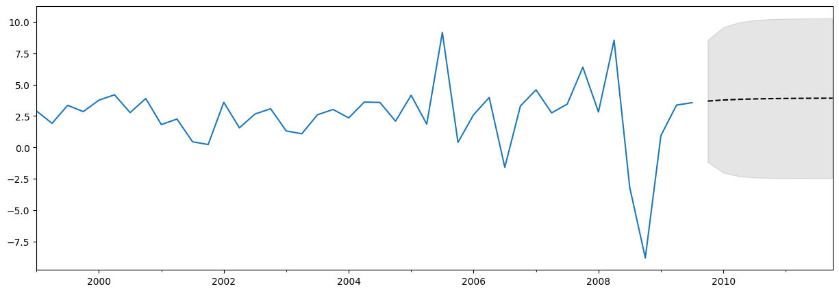
通常绘制数据、预测值和置信区间是很有用的。有很多方法可以做到这一点,但这里有一个示例
[10]:
fig, ax = plt.subplots(figsize=(15, 5))

# Plot the data (here we are subsetting it to get a better look at the forecasts)
endog.loc['1999':].plot(ax=ax)

# Construct the forecasts
fcast = res.get_forecast('2011Q4').summary_frame()
fcast['mean'].plot(ax=ax, style='k--')
ax.fill_between(fcast.index, fcast['mean_ci_lower'], fcast['mean_ci_upper'], color='k', alpha=0.1);
关于预测结果的说明
上面的预测可能看起来并不令人印象深刻,因为它几乎是一条直线。这是因为这是一个非常简单的单变量预测模型。尽管如此,请记住,这些简单的预测模型可以极具竞争力。
预测与预报
结果对象还包含两个方法,允许进行样本内拟合值和样本外预测。它们是 predict 和 get_prediction。predict 方法仅返回点预测(类似于 forecast),而 get_prediction 方法还返回附加结果(类似于 get_forecast)。
一般来说,如果你的兴趣是样本外预测,使用forecast和get_forecast方法会更简单。
交叉验证
注意:本节中使用的一些函数是在 statsmodels v0.11.0 中首次引入的。
一个常见的用例是通过递归地执行h步预测来进行预测方法的交叉验证,使用以下过程:
在训练样本上拟合模型参数
从样本末尾生成h步提前预测
将预测结果与测试数据集进行比较以计算错误率
扩展示例以包含下一个观测值,并重复
经济学家有时称这为伪样本外预测评估练习,或时间序列交叉验证。
示例
我们将使用上述通货膨胀数据集进行一个非常简单的练习。完整的数据集包含203个观测值,为了说明目的,我们将使用前80%作为我们的训练样本,并且只考虑一步预测。
上述过程的单次迭代如下所示:
[11]:
# Step 1: fit model parameters w/ training sample
training_obs = int(len(endog) * 0.8)

training_endog = endog[:training_obs]
training_mod = sm.tsa.SARIMAX(
    training_endog, order=(1, 0, 0), trend='c')
training_res = training_mod.fit()

# Print the estimated parameters
print(training_res.params)
intercept    1.162076
ar.L1        0.724242
sigma2       5.051600
dtype: float64
[12]:
# Step 2: produce one-step-ahead forecasts
fcast = training_res.forecast()

# Step 3: compute root mean square forecasting error
true = endog.reindex(fcast.index)
error = true - fcast

# Print out the results
print(pd.concat([true.rename('true'),
                 fcast.rename('forecast'),
                 error.rename('error')], axis=1))
        true  forecast    error
1999Q3  3.35   2.55262  0.79738
要添加另一个观察结果,我们可以使用 append 或 extend 结果方法。这两种方法都可以产生相同的预测,但它们在其他可用的结果上有所不同:
append是一个更完整的方法。它总是为所有训练观察结果存储结果,并且可以选择性地根据新观察结果重新拟合模型参数(请注意,默认情况下不重新拟合参数)。extend是一种更快速的方法,如果训练样本非常大,可能会很有用。它仅存储新观测值的结果,并且不允许重新拟合模型参数(即你必须使用在前一个样本上估计的参数)。
如果你的训练样本相对较小(例如,少于几千个观测值),或者如果你想计算最佳的预测,那么你应该使用append方法。然而,如果该方法不可行(例如,因为你有一个非常大的训练样本),或者如果你可以接受稍微次优的预测(因为参数估计会稍微过时),那么你可以考虑使用extend方法。
第二次迭代,使用append方法并重新拟合参数,步骤如下(再次注意,append的默认设置不会重新拟合参数,但我们通过refit=True参数覆盖了这一点):
[13]:
# Step 1: append a new observation to the sample and refit the parameters
append_res = training_res.append(endog[training_obs:training_obs + 1], refit=True)

# Print the re-estimated parameters
print(append_res.params)
intercept    1.171544
ar.L1        0.723152
sigma2       5.024580
dtype: float64
请注意,这些估计的参数与我们最初估计的参数略有不同。通过新的结果对象append_res,我们可以从比之前的调用多一个观测值的位置开始计算预测:
[14]:
# Step 2: produce one-step-ahead forecasts
fcast = append_res.forecast()

# Step 3: compute root mean square forecasting error
true = endog.reindex(fcast.index)
error = true - fcast

# Print out the results
print(pd.concat([true.rename('true'),
                 fcast.rename('forecast'),
                 error.rename('error')], axis=1))
        true  forecast     error
1999Q4  2.85  3.594102 -0.744102
综上所述,我们可以按照以下步骤进行递归预测评估练习:
[15]:
# Setup forecasts
nforecasts = 3
forecasts = {}

# Get the number of initial training observations
nobs = len(endog)
n_init_training = int(nobs * 0.8)

# Create model for initial training sample, fit parameters
init_training_endog = endog.iloc[:n_init_training]
mod = sm.tsa.SARIMAX(training_endog, order=(1, 0, 0), trend='c')
res = mod.fit()

# Save initial forecast
forecasts[training_endog.index[-1]] = res.forecast(steps=nforecasts)

# Step through the rest of the sample
for t in range(n_init_training, nobs):
    # Update the results by appending the next observation
    updated_endog = endog.iloc[t:t+1]
    res = res.append(updated_endog, refit=False)

    # Save the new set of forecasts
    forecasts[updated_endog.index[0]] = res.forecast(steps=nforecasts)

# Combine all forecasts into a dataframe
forecasts = pd.concat(forecasts, axis=1)

print(forecasts.iloc[:5, :5])
          1999Q2    1999Q3    1999Q4    2000Q1    2000Q2
1999Q3  2.552620       NaN       NaN       NaN       NaN
1999Q4  3.010790  3.588286       NaN       NaN       NaN
2000Q1  3.342616  3.760863  3.226165       NaN       NaN
2000Q2       NaN  3.885850  3.498599  3.885225       NaN
2000Q3       NaN       NaN  3.695908  3.975918  4.196649
我们现在有一组在每个时间点从1999年第二季度到2009年第三季度做出的三个预测。我们可以通过从该点的endog实际值中减去每个预测来构建预测误差。
[16]:
# Construct the forecast errors
forecast_errors = forecasts.apply(lambda column: endog - column).reindex(forecasts.index)

print(forecast_errors.iloc[:5, :5])
          1999Q2    1999Q3    1999Q4    2000Q1    2000Q2
1999Q3  0.797380       NaN       NaN       NaN       NaN
1999Q4 -0.160790 -0.738286       NaN       NaN       NaN
2000Q1  0.417384 -0.000863  0.533835       NaN       NaN
2000Q2       NaN  0.304150  0.691401  0.304775       NaN
2000Q3       NaN       NaN -0.925908 -1.205918 -1.426649
为了评估我们的预测,我们通常希望查看一个汇总值,如均方根误差。在这里,我们可以通过首先将预测误差展平,使它们按时间范围索引,然后为每个时间范围计算均方根误差。
[17]:
# Reindex the forecasts by horizon rather than by date
def flatten(column):
    return column.dropna().reset_index(drop=True)

flattened = forecast_errors.apply(flatten)
flattened.index = (flattened.index + 1).rename('horizon')

print(flattened.iloc[:3, :5])
           1999Q2    1999Q3    1999Q4    2000Q1    2000Q2
horizon
1        0.797380 -0.738286  0.533835  0.304775 -1.426649
2       -0.160790 -0.000863  0.691401 -1.205918 -0.311464
3        0.417384  0.304150 -0.925908 -0.151602 -2.384952
[18]:
# Compute the root mean square error
rmse = (flattened**2).mean(axis=1)**0.5

print(rmse)
horizon
1    3.292700
2    3.421808
3    3.280012
dtype: float64
使用 extend
如果我们使用extend方法,我们可以检查是否得到类似的预测,但它们并不完全相同于我们使用append方法并设置refit=True参数时的情况。这是因为extend方法不会根据新观测值重新估计参数。
[19]:
# Setup forecasts
nforecasts = 3
forecasts = {}

# Get the number of initial training observations
nobs = len(endog)
n_init_training = int(nobs * 0.8)

# Create model for initial training sample, fit parameters
init_training_endog = endog.iloc[:n_init_training]
mod = sm.tsa.SARIMAX(training_endog, order=(1, 0, 0), trend='c')
res = mod.fit()

# Save initial forecast
forecasts[training_endog.index[-1]] = res.forecast(steps=nforecasts)

# Step through the rest of the sample
for t in range(n_init_training, nobs):
    # Update the results by appending the next observation
    updated_endog = endog.iloc[t:t+1]
    res = res.extend(updated_endog)

    # Save the new set of forecasts
    forecasts[updated_endog.index[0]] = res.forecast(steps=nforecasts)

# Combine all forecasts into a dataframe
forecasts = pd.concat(forecasts, axis=1)

print(forecasts.iloc[:5, :5])
          1999Q2    1999Q3    1999Q4    2000Q1    2000Q2
1999Q3  2.552620       NaN       NaN       NaN       NaN
1999Q4  3.010790  3.588286       NaN       NaN       NaN
2000Q1  3.342616  3.760863  3.226165       NaN       NaN
2000Q2       NaN  3.885850  3.498599  3.885225       NaN
2000Q3       NaN       NaN  3.695908  3.975918  4.196649
[20]:
# Construct the forecast errors
forecast_errors = forecasts.apply(lambda column: endog - column).reindex(forecasts.index)

print(forecast_errors.iloc[:5, :5])
          1999Q2    1999Q3    1999Q4    2000Q1    2000Q2
1999Q3  0.797380       NaN       NaN       NaN       NaN
1999Q4 -0.160790 -0.738286       NaN       NaN       NaN
2000Q1  0.417384 -0.000863  0.533835       NaN       NaN
2000Q2       NaN  0.304150  0.691401  0.304775       NaN
2000Q3       NaN       NaN -0.925908 -1.205918 -1.426649
[21]:
# Reindex the forecasts by horizon rather than by date
def flatten(column):
    return column.dropna().reset_index(drop=True)

flattened = forecast_errors.apply(flatten)
flattened.index = (flattened.index + 1).rename('horizon')

print(flattened.iloc[:3, :5])
           1999Q2    1999Q3    1999Q4    2000Q1    2000Q2
horizon
1        0.797380 -0.738286  0.533835  0.304775 -1.426649
2       -0.160790 -0.000863  0.691401 -1.205918 -0.311464
3        0.417384  0.304150 -0.925908 -0.151602 -2.384952
[22]:
# Compute the root mean square error
rmse = (flattened**2).mean(axis=1)**0.5

print(rmse)
horizon
1    3.292700
2    3.421808
3    3.280012
dtype: float64
通过不重新估计参数,我们的预测略差(每个时间段的均方根误差更高)。然而,这个过程更快,即使只有200个数据点。使用%%timeit单元魔法对上述单元进行计时,我们发现使用extend的运行时间为570毫秒,而使用append并设置refit=True的运行时间为1.7秒。(请注意,使用extend也比使用append并设置refit=False更快)。
索引
在本笔记本中,我们一直在使用带有相关频率的Pandas日期索引。正如您所见,此索引将我们的数据标记为季度频率,时间范围从1959年第一季度到2009年第三季度。
[23]:
print(endog.index)
PeriodIndex(['1959Q1', '1959Q2', '1959Q3', '1959Q4', '1960Q1', '1960Q2',
             '1960Q3', '1960Q4', '1961Q1', '1961Q2',
             ...
             '2007Q2', '2007Q3', '2007Q4', '2008Q1', '2008Q2', '2008Q3',
             '2008Q4', '2009Q1', '2009Q2', '2009Q3'],
            dtype='period[Q-DEC]', length=203)
在大多数情况下,如果你的数据有一个带有定义频率(如季度、月度等)的日期/时间索引,那么最好确保你的数据是一个带有适当索引的Pandas系列。以下是三个示例:
[24]:
# Annual frequency, using a PeriodIndex
index = pd.period_range(start='2000', periods=4, freq='Y')
endog1 = pd.Series([1, 2, 3, 4], index=index)
print(endog1.index)
PeriodIndex(['2000', '2001', '2002', '2003'], dtype='period[Y-DEC]')
[25]:
# Quarterly frequency, using a DatetimeIndex
index = pd.date_range(start='2000', periods=4, freq='QS')
endog2 = pd.Series([1, 2, 3, 4], index=index)
print(endog2.index)
DatetimeIndex(['2000-01-01', '2000-04-01', '2000-07-01', '2000-10-01'], dtype='datetime64[ns]', freq='QS-JAN')
[26]:
# Monthly frequency, using a DatetimeIndex
index = pd.date_range(start='2000', periods=4, freq='ME')
endog3 = pd.Series([1, 2, 3, 4], index=index)
print(endog3.index)
DatetimeIndex(['2000-01-31', '2000-02-29', '2000-03-31', '2000-04-30'], dtype='datetime64[ns]', freq='ME')
事实上,如果你的数据有一个关联的日期/时间索引,即使它没有定义的频率,最好还是使用它。以下是这种索引的一个例子——注意它有freq=None:
[27]:
index = pd.DatetimeIndex([
    '2000-01-01 10:08am', '2000-01-01 11:32am',
    '2000-01-01 5:32pm', '2000-01-02 6:15am'])
endog4 = pd.Series([0.2, 0.5, -0.1, 0.1], index=index)
print(endog4.index)
DatetimeIndex(['2000-01-01 10:08:00', '2000-01-01 11:32:00',
               '2000-01-01 17:32:00', '2000-01-02 06:15:00'],
              dtype='datetime64[ns]', freq=None)
您仍然可以将此数据传递给 statsmodels 的模型类,但您将收到以下警告,即未找到频率数据:
[28]:
mod = sm.tsa.SARIMAX(endog4)
res = mod.fit()
/Users/cw/baidu/code/fin_tool/github/statsmodels/venv/lib/python3.11/site-packages/statsmodels/tsa/base/tsa_model.py:473: ValueWarning: A date index has been provided, but it has no associated frequency information and so will be ignored when e.g. forecasting.
  self._init_dates(dates, freq)
/Users/cw/baidu/code/fin_tool/github/statsmodels/venv/lib/python3.11/site-packages/statsmodels/tsa/base/tsa_model.py:473: ValueWarning: A date index has been provided, but it has no associated frequency information and so will be ignored when e.g. forecasting.
  self._init_dates(dates, freq)
这意味着您不能通过日期指定预测步骤,并且 forecast 和 get_forecast 方法的输出将不会有关联的日期。原因是,如果没有给定的频率,就无法确定每个预测应分配到哪个日期。在上面的例子中,索引的日期/时间戳没有模式,因此无法确定下一个日期/时间应该是什么(应该是2000-01-02的早晨?下午?还是可能要到2000-01-03?)。
例如,如果我们进行一步预测:
[29]:
res.forecast(1)
/Users/cw/baidu/code/fin_tool/github/statsmodels/venv/lib/python3.11/site-packages/statsmodels/tsa/base/tsa_model.py:837: ValueWarning: No supported index is available. Prediction results will be given with an integer index beginning at `start`.
  return get_prediction_index(
/Users/cw/baidu/code/fin_tool/github/statsmodels/venv/lib/python3.11/site-packages/statsmodels/tsa/base/tsa_model.py:837: FutureWarning: No supported index is available. In the next version, calling this method in a model without a supported index will result in an exception.
  return get_prediction_index(
[29]:
4    0.011866
dtype: float64
与新预测相关联的索引是 4,因为如果给定的数据具有整数索引,那么这将是下一个值。系统会发出警告,告知用户该索引不是日期/时间索引。
如果我们尝试使用日期来指定预测的步骤,将会得到以下异常:
KeyError: 'The `end` argument could not be matched to a location related to the index of the data.'
[30]:
# Here we'll catch the exception to prevent printing too much of
# the exception trace output in this notebook
try:
    res.forecast('2000-01-03')
except KeyError as e:
    print(e)
'The `end` argument could not be matched to a location related to the index of the data.'
最终,使用没有关联的日期/时间频率的数据,甚至使用完全没有索引的数据,比如Numpy数组,并没有什么问题。然而,如果你可以使用带有关联频率的Pandas系列,你将有更多的选项来指定你的预测,并获得带有更有用索引的结果。