比较结合过采样和欠采样的采样器

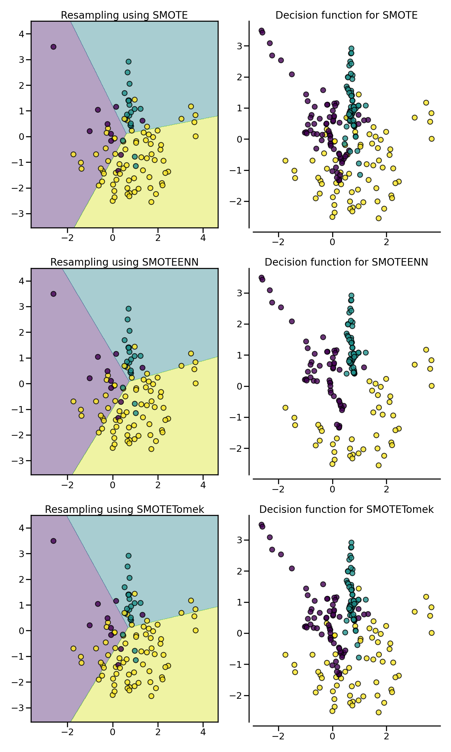
此示例展示了在SMOTE过采样后应用欠采样算法的效果。在文献中，Tomek's link和编辑最近邻是两种已被使用并在imbalanced-learn中可用的方法。

# Authors: Guillaume Lemaitre <g.lemaitre58@gmail.com>
# License: MIT

print(__doc__)

import matplotlib.pyplot as plt
import seaborn as sns

sns.set_context("poster")

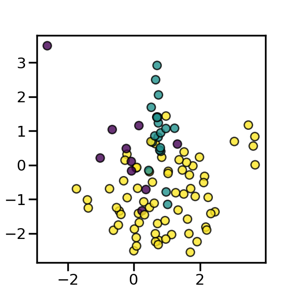
数据集生成

我们将创建一个包含几个样本的不平衡数据集。我们将使用 make_classification 来生成这个数据集。

from sklearn.datasets import make_classification

X, y = make_classification(
    n_samples=100,
    n_features=2,
    n_informative=2,
    n_redundant=0,
    n_repeated=0,
    n_classes=3,
    n_clusters_per_class=1,
    weights=[0.1, 0.2, 0.7],
    class_sep=0.8,
    random_state=0,
)

_, ax = plt.subplots(figsize=(6, 6))
_ = ax.scatter(X[:, 0], X[:, 1], c=y, alpha=0.8, edgecolor="k")

以下函数将用于绘制重采样后的样本空间，以说明算法的特性。

from collections import Counter


def plot_resampling(X, y, sampler, ax):
    """Plot the resampled dataset using the sampler."""
    X_res, y_res = sampler.fit_resample(X, y)
    ax.scatter(X_res[:, 0], X_res[:, 1], c=y_res, alpha=0.8, edgecolor="k")
    sns.despine(ax=ax, offset=10)
    ax.set_title(f"Decision function for {sampler.__class__.__name__}")
    return Counter(y_res)

以下函数将用于绘制给定一些数据的分类器的决策函数。

import numpy as np


def plot_decision_function(X, y, clf, ax):
    """Plot the decision function of the classifier and the original data"""
    plot_step = 0.02
    x_min, x_max = X[:, 0].min() - 1, X[:, 0].max() + 1
    y_min, y_max = X[:, 1].min() - 1, X[:, 1].max() + 1
    xx, yy = np.meshgrid(
        np.arange(x_min, x_max, plot_step), np.arange(y_min, y_max, plot_step)
    )

    Z = clf.predict(np.c_[xx.ravel(), yy.ravel()])
    Z = Z.reshape(xx.shape)
    ax.contourf(xx, yy, Z, alpha=0.4)
    ax.scatter(X[:, 0], X[:, 1], alpha=0.8, c=y, edgecolor="k")
    ax.set_title(f"Resampling using {clf[0].__class__.__name__}")

SMOTE 允许生成样本。然而，这种过采样方法对底层分布没有任何了解。因此，可能会生成一些噪声样本，例如当不同类别无法很好分离时。因此，应用欠采样算法来清理噪声样本可能是有益的。文献中通常使用两种方法：(i) Tomek’s link 和 (ii) 编辑最近邻清理方法。Imbalanced-learn 提供了两种现成的采样器 SMOTETomek 和 SMOTEENN。通常，SMOTEENN 比 SMOTETomek 清理更多的噪声数据。

from sklearn.linear_model import LogisticRegression

from imblearn.combine import SMOTEENN, SMOTETomek

from imblearn.over_sampling import SMOTE
from imblearn.pipeline import make_pipeline

samplers = [SMOTE(random_state=0), SMOTEENN(random_state=0), SMOTETomek(random_state=0)]

fig, axs = plt.subplots(3, 2, figsize=(15, 25))
for ax, sampler in zip(axs, samplers):
    clf = make_pipeline(sampler, LogisticRegression()).fit(X, y)
    plot_decision_function(X, y, clf, ax[0])
    plot_resampling(X, y, sampler, ax[1])
fig.tight_layout()

plt.show()

预计内存使用量： 199 MB