注意

Go to the end 以下载完整的示例代码。

比较过采样采样器#

以下示例旨在对不平衡学习包中提供的不同过采样算法进行定性比较。

# Authors: Guillaume Lemaitre <g.lemaitre58@gmail.com>
# License: MIT

print(__doc__)

import matplotlib.pyplot as plt
import seaborn as sns

sns.set_context("poster")

以下函数将用于创建玩具数据集。它使用了来自scikit-learn的make_classification，但固定了一些参数。

from sklearn.datasets import make_classification


def create_dataset(
    n_samples=1000,
    weights=(0.01, 0.01, 0.98),
    n_classes=3,
    class_sep=0.8,
    n_clusters=1,
):
    return make_classification(
        n_samples=n_samples,
        n_features=2,
        n_informative=2,
        n_redundant=0,
        n_repeated=0,
        n_classes=n_classes,
        n_clusters_per_class=n_clusters,
        weights=list(weights),
        class_sep=class_sep,
        random_state=0,
    )

以下函数将用于绘制重采样后的样本空间，以说明算法的特性。

def plot_resampling(X, y, sampler, ax, title=None):
    X_res, y_res = sampler.fit_resample(X, y)
    ax.scatter(X_res[:, 0], X_res[:, 1], c=y_res, alpha=0.8, edgecolor="k")
    if title is None:
        title = f"Resampling with {sampler.__class__.__name__}"
    ax.set_title(title)
    sns.despine(ax=ax, offset=10)

以下函数将用于绘制给定一些数据的分类器的决策函数。

import numpy as np


def plot_decision_function(X, y, clf, ax, title=None):
    plot_step = 0.02
    x_min, x_max = X[:, 0].min() - 1, X[:, 0].max() + 1
    y_min, y_max = X[:, 1].min() - 1, X[:, 1].max() + 1
    xx, yy = np.meshgrid(
        np.arange(x_min, x_max, plot_step), np.arange(y_min, y_max, plot_step)
    )

    Z = clf.predict(np.c_[xx.ravel(), yy.ravel()])
    Z = Z.reshape(xx.shape)
    ax.contourf(xx, yy, Z, alpha=0.4)
    ax.scatter(X[:, 0], X[:, 1], alpha=0.8, c=y, edgecolor="k")
    if title is not None:
        ax.set_title(title)

平衡比率影响的图示#

我们将首先使用逻辑回归分类器（一种线性模型）来说明平衡比例对某些玩具数据的影响。

from sklearn.linear_model import LogisticRegression

clf = LogisticRegression()

我们将拟合并展示决策边界模型，以说明处理不平衡类别的影响。

fig, axs = plt.subplots(nrows=2, ncols=2, figsize=(15, 12))

weights_arr = (
    (0.01, 0.01, 0.98),
    (0.01, 0.05, 0.94),
    (0.2, 0.1, 0.7),
    (0.33, 0.33, 0.33),
)
for ax, weights in zip(axs.ravel(), weights_arr):
    X, y = create_dataset(n_samples=300, weights=weights)
    clf.fit(X, y)
    plot_decision_function(X, y, clf, ax, title=f"weight={weights}")
    fig.suptitle(f"Decision function of {clf.__class__.__name__}")
fig.tight_layout()

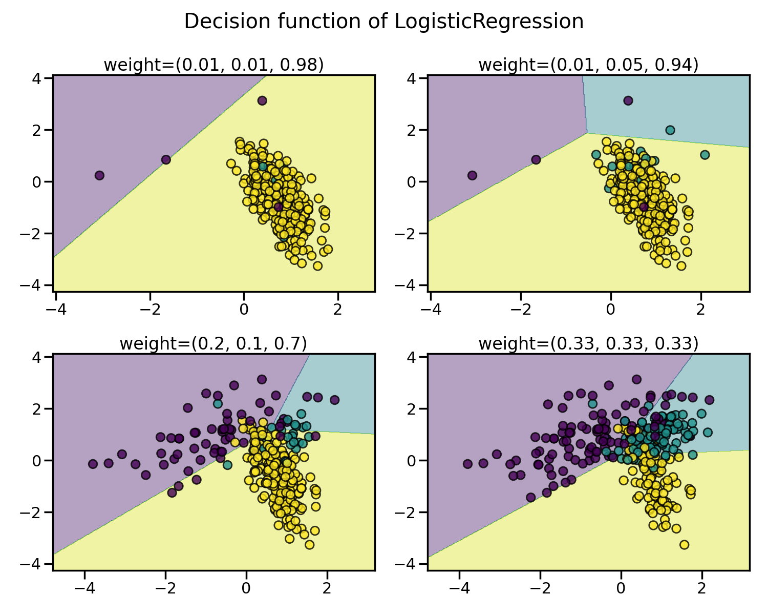
Decision function of LogisticRegression, weight=(0.01, 0.01, 0.98), weight=(0.01, 0.05, 0.94), weight=(0.2, 0.1, 0.7), weight=(0.33, 0.33, 0.33)

每个类别中的样本数量差异越大，分类结果越差。

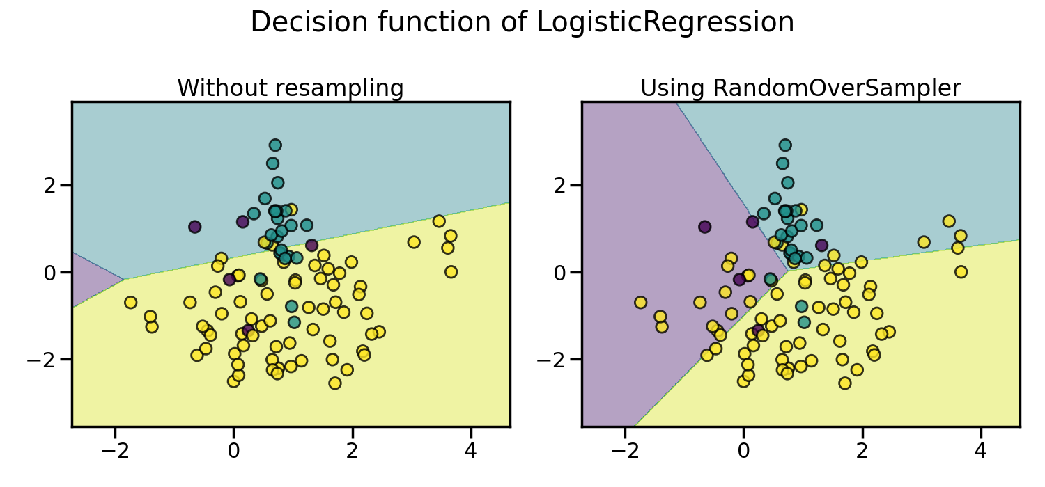
随机过采样以平衡数据集#

随机过采样可以用于重复一些样本并平衡数据集中的样本数量。可以看出，使用这种简单的方法，决策边界已经不再偏向多数类。类 RandomOverSampler 实现了这种策略。

from imblearn.over_sampling import RandomOverSampler

from imblearn.pipeline import make_pipeline

X, y = create_dataset(n_samples=100, weights=(0.05, 0.25, 0.7))

fig, axs = plt.subplots(nrows=1, ncols=2, figsize=(15, 7))

clf.fit(X, y)
plot_decision_function(X, y, clf, axs[0], title="Without resampling")

sampler = RandomOverSampler(random_state=0)
model = make_pipeline(sampler, clf).fit(X, y)
plot_decision_function(X, y, model, axs[1], f"Using {model[0].__class__.__name__}")

fig.suptitle(f"Decision function of {clf.__class__.__name__}")
fig.tight_layout()

Decision function of LogisticRegression, Without resampling, Using RandomOverSampler

默认情况下，随机过采样会生成一个引导样本。参数 shrinkage 允许对生成的数据添加一个小扰动，以生成平滑的引导样本。下图显示了两种数据生成策略之间的差异。

fig, axs = plt.subplots(nrows=1, ncols=2, figsize=(15, 7))

sampler.set_params(shrinkage=None)
plot_resampling(X, y, sampler, ax=axs[0], title="Normal bootstrap")

sampler.set_params(shrinkage=0.3)
plot_resampling(X, y, sampler, ax=axs[1], title="Smoothed bootstrap")

fig.suptitle(f"Resampling with {sampler.__class__.__name__}")
fig.tight_layout()

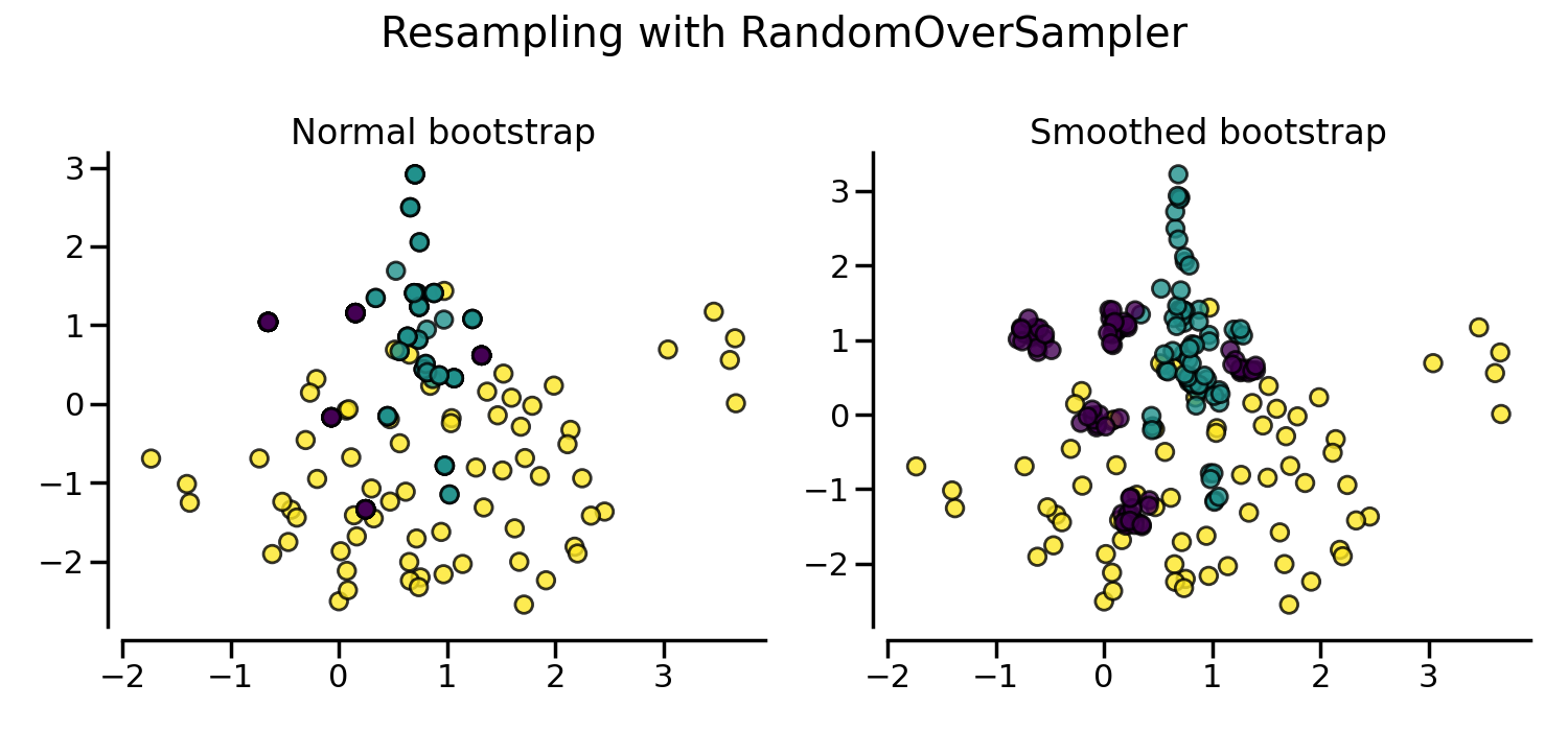
Resampling with RandomOverSampler, Normal bootstrap, Smoothed bootstrap

看起来使用平滑自举法生成了更多的样本。这是由于生成的样本没有与原始样本叠加。

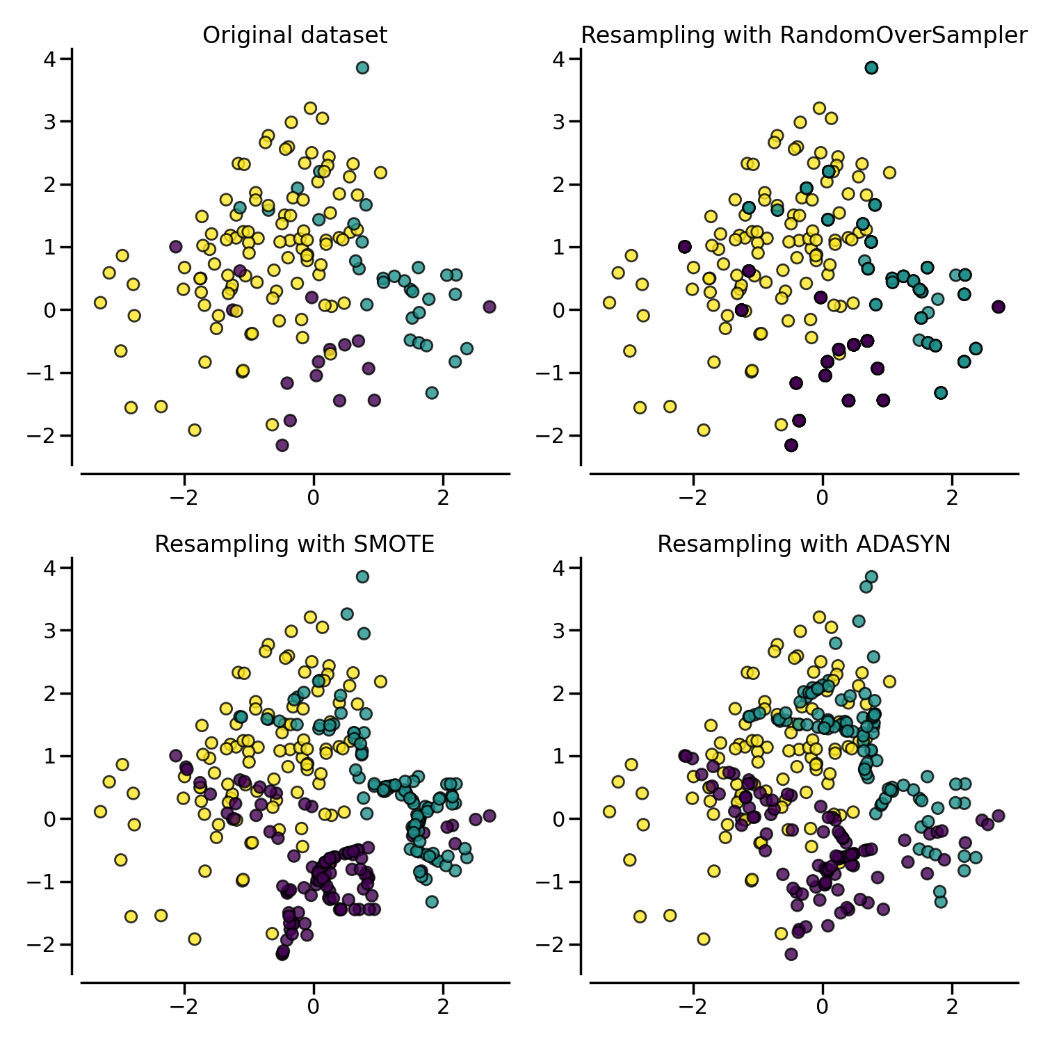
使用ADASYN和SMOTE进行更高级的过采样#

在过采样或扰动生成的引导样本时，可以使用一些特定的启发式方法，而不是重复相同的样本。ADASYN 和 SMOTE 在这种情况下可以使用。

from imblearn import FunctionSampler  # to use a idendity sampler
from imblearn.over_sampling import ADASYN, SMOTE

X, y = create_dataset(n_samples=150, weights=(0.1, 0.2, 0.7))

fig, axs = plt.subplots(nrows=2, ncols=2, figsize=(15, 15))

samplers = [
    FunctionSampler(),
    RandomOverSampler(random_state=0),
    SMOTE(random_state=0),
    ADASYN(random_state=0),
]

for ax, sampler in zip(axs.ravel(), samplers):
    title = "Original dataset" if isinstance(sampler, FunctionSampler) else None
    plot_resampling(X, y, sampler, ax, title=title)
fig.tight_layout()

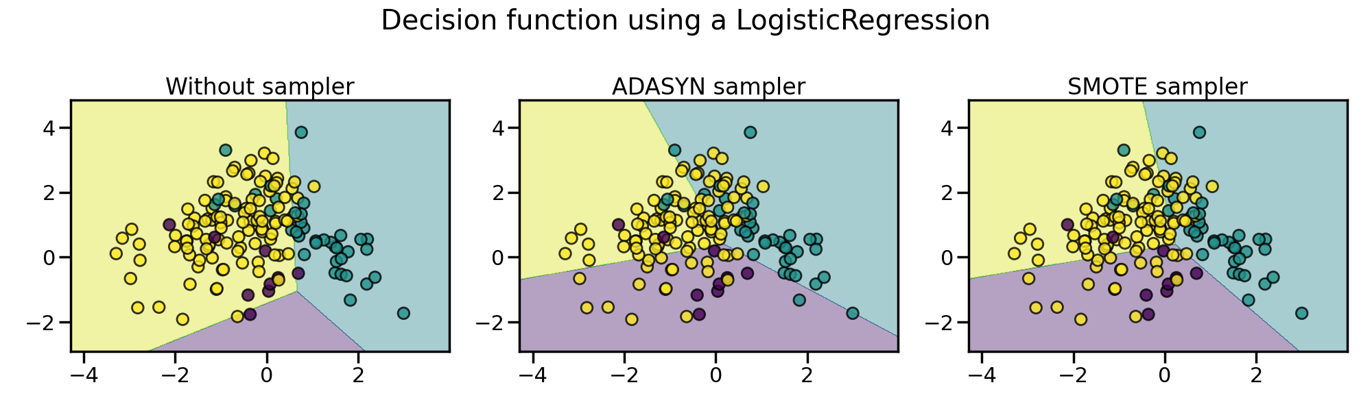
Original dataset, Resampling with RandomOverSampler, Resampling with SMOTE, Resampling with ADASYN

以下图表展示了 ADASYN 和 SMOTE 之间的区别。 ADASYN 将专注于那些难以通过最近邻规则分类的样本，而常规的 SMOTE 则不会做出任何区分。因此，决策函数取决于所使用的算法。

X, y = create_dataset(n_samples=150, weights=(0.05, 0.25, 0.7))

fig, axs = plt.subplots(nrows=1, ncols=3, figsize=(20, 6))

models = {
    "Without sampler": clf,
    "ADASYN sampler": make_pipeline(ADASYN(random_state=0), clf),
    "SMOTE sampler": make_pipeline(SMOTE(random_state=0), clf),
}

for ax, (title, model) in zip(axs, models.items()):
    model.fit(X, y)
    plot_decision_function(X, y, model, ax=ax, title=title)

fig.suptitle(f"Decision function using a {clf.__class__.__name__}")
fig.tight_layout()

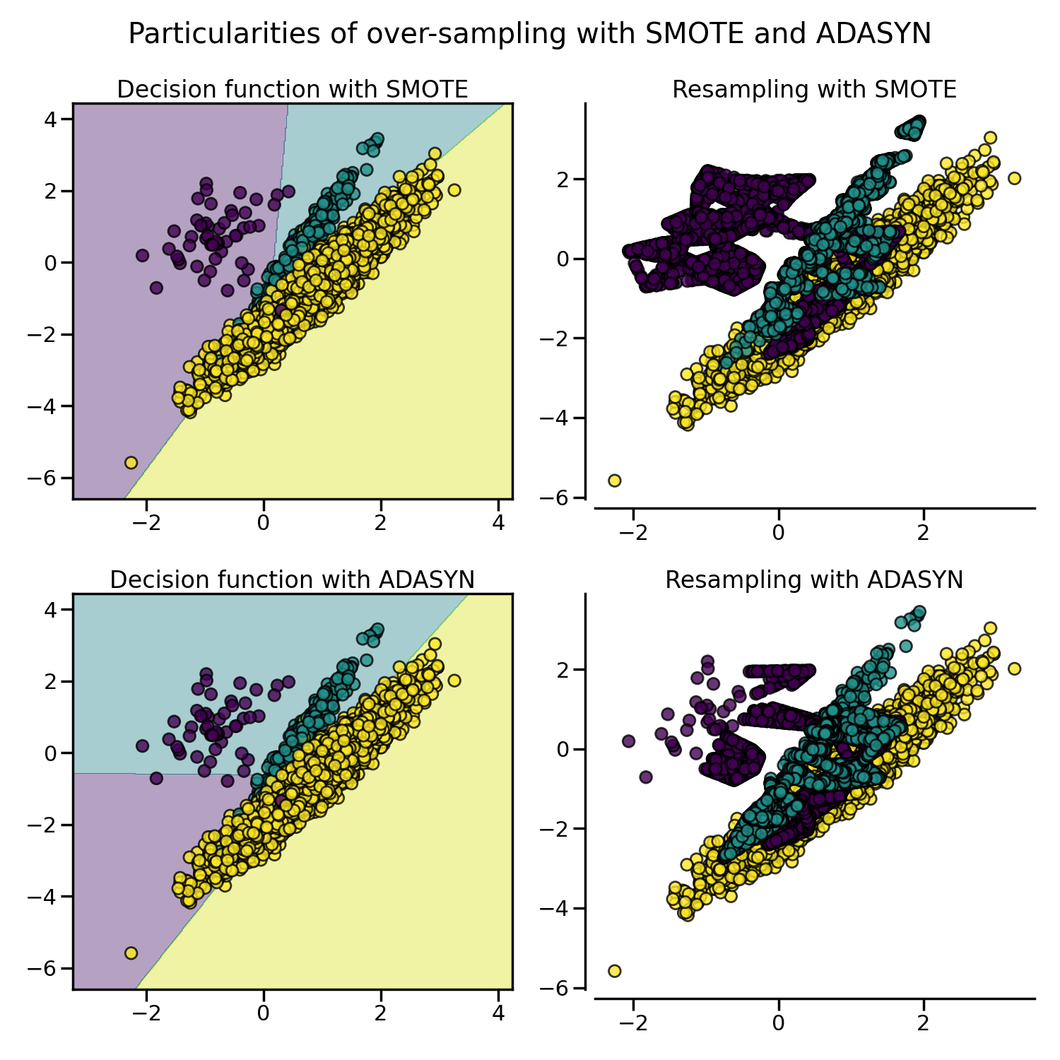
Decision function using a LogisticRegression, Without sampler, ADASYN sampler, SMOTE sampler

由于这些采样的特殊性，它可能会引发一些特定的问题，如下所示。

X, y = create_dataset(n_samples=5000, weights=(0.01, 0.05, 0.94), class_sep=0.8)

samplers = [SMOTE(random_state=0), ADASYN(random_state=0)]

fig, axs = plt.subplots(nrows=2, ncols=2, figsize=(15, 15))
for ax, sampler in zip(axs, samplers):
    model = make_pipeline(sampler, clf).fit(X, y)
    plot_decision_function(
        X, y, clf, ax[0], title=f"Decision function with {sampler.__class__.__name__}"
    )
    plot_resampling(X, y, sampler, ax[1])

fig.suptitle("Particularities of over-sampling with SMOTE and ADASYN")
fig.tight_layout()

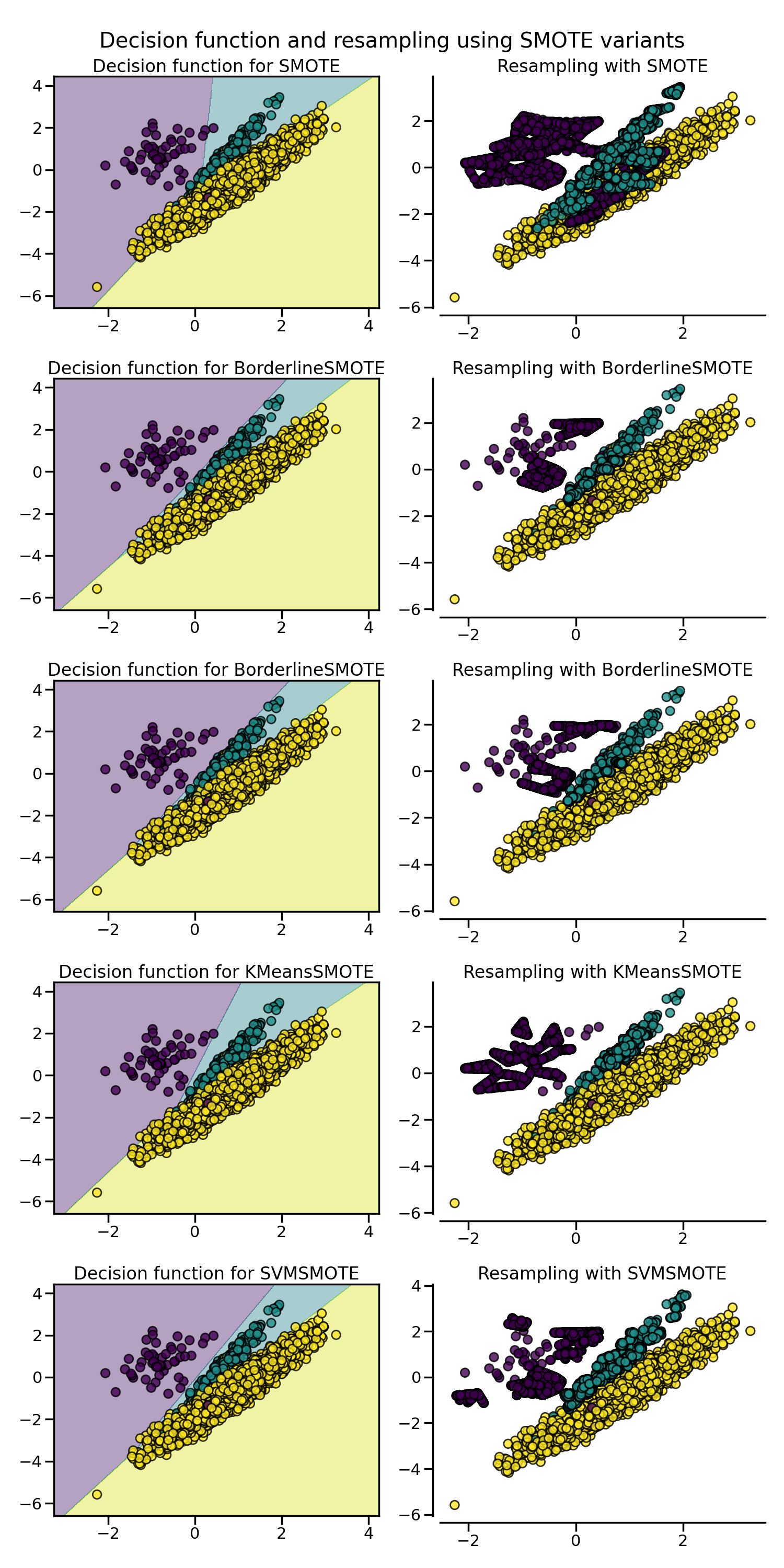
Particularities of over-sampling with SMOTE and ADASYN, Decision function with SMOTE, Resampling with SMOTE, Decision function with ADASYN, Resampling with ADASYN

SMOTE 提出了几种变体，通过在重采样过程中识别特定样本。边界版本 (BorderlineSMOTE) 将检测哪些点位于两个类之间的边界上。SVM 版本 (SVMSMOTE) 将使用通过 SVM 算法找到的支持向量来创建新样本，而 KMeans 版本 (KMeansSMOTE) 将在生成样本之前进行聚类，根据每个簇的密度独立生成样本。

from sklearn.cluster import MiniBatchKMeans

from imblearn.over_sampling import SVMSMOTE, BorderlineSMOTE, KMeansSMOTE

X, y = create_dataset(n_samples=5000, weights=(0.01, 0.05, 0.94), class_sep=0.8)

fig, axs = plt.subplots(5, 2, figsize=(15, 30))

samplers = [
    SMOTE(random_state=0),
    BorderlineSMOTE(random_state=0, kind="borderline-1"),
    BorderlineSMOTE(random_state=0, kind="borderline-2"),
    KMeansSMOTE(
        kmeans_estimator=MiniBatchKMeans(n_clusters=10, n_init=1, random_state=0),
        random_state=0,
    ),
    SVMSMOTE(random_state=0),
]

for ax, sampler in zip(axs, samplers):
    model = make_pipeline(sampler, clf).fit(X, y)
    plot_decision_function(
        X, y, clf, ax[0], title=f"Decision function for {sampler.__class__.__name__}"
    )
    plot_resampling(X, y, sampler, ax[1])

fig.suptitle("Decision function and resampling using SMOTE variants")
fig.tight_layout()

Decision function and resampling using SMOTE variants, Decision function for SMOTE, Resampling with SMOTE, Decision function for BorderlineSMOTE, Resampling with BorderlineSMOTE, Decision function for BorderlineSMOTE, Resampling with BorderlineSMOTE, Decision function for KMeansSMOTE, Resampling with KMeansSMOTE, Decision function for SVMSMOTE, Resampling with SVMSMOTE

当处理连续和分类特征的混合时， SMOTENC 是唯一可以处理这种情况的方法。

from collections import Counter

from imblearn.over_sampling import SMOTENC

rng = np.random.RandomState(42)
n_samples = 50
# Create a dataset of a mix of numerical and categorical data
X = np.empty((n_samples, 3), dtype=object)
X[:, 0] = rng.choice(["A", "B", "C"], size=n_samples).astype(object)
X[:, 1] = rng.randn(n_samples)
X[:, 2] = rng.randint(3, size=n_samples)
y = np.array([0] * 20 + [1] * 30)

print("The original imbalanced dataset")
print(sorted(Counter(y).items()))
print()
print("The first and last columns are containing categorical features:")
print(X[:5])
print()

smote_nc = SMOTENC(categorical_features=[0, 2], random_state=0)
X_resampled, y_resampled = smote_nc.fit_resample(X, y)
print("Dataset after resampling:")
print(sorted(Counter(y_resampled).items()))
print()
print("SMOTE-NC will generate categories for the categorical features:")
print(X_resampled[-5:])
print()

The original imbalanced dataset
[(0, 20), (1, 30)]

The first and last columns are containing categorical features:
[['C' -0.14021849735700803 2]
 ['A' -0.033193400066544886 2]
 ['C' -0.7490765234433554 1]
 ['C' -0.7783820070908942 2]
 ['A' 0.948842857719016 2]]

Dataset after resampling:
[(0, 30), (1, 30)]

SMOTE-NC will generate categories for the categorical features:
[['A' 0.1989993778979113 2]
 ['B' -0.3657680728116921 2]
 ['B' 0.8790828729585258 2]
 ['B' 0.3710891618824609 2]
 ['B' 0.3327240726719727 2]]

然而，如果数据集仅由分类特征组成，则应使用SMOTEN。

from imblearn.over_sampling import SMOTEN

# Generate only categorical data
X = np.array(["A"] * 10 + ["B"] * 20 + ["C"] * 30, dtype=object).reshape(-1, 1)
y = np.array([0] * 20 + [1] * 40, dtype=np.int32)

print(f"Original class counts: {Counter(y)}")
print()
print(X[:5])
print()

sampler = SMOTEN(random_state=0)
X_res, y_res = sampler.fit_resample(X, y)
print(f"Class counts after resampling {Counter(y_res)}")
print()
print(X_res[-5:])
print()

Original class counts: Counter({1: 40, 0: 20})

[['A']
 ['A']
 ['A']
 ['A']
 ['A']]

Class counts after resampling Counter({0: 40, 1: 40})

[['B']
 ['B']
 ['A']
 ['B']
 ['A']]

脚本的总运行时间： (0 分钟 11.991 秒)

预计内存使用量： 321 MB

图库由Sphinx-Gallery生成

比较过采样采样器#

平衡比率影响的图示#

随机过采样以平衡数据集#

使用ADASYN和SMOTE进行更高级的过采样#

本页面