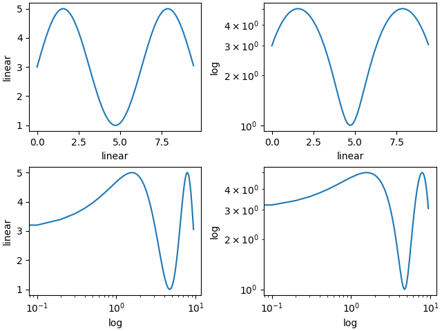
轴刻度

默认情况下，Matplotlib 在轴上使用线性刻度显示数据。Matplotlib 还支持 对数刻度，以及其他一些不太常见的刻度。通常可以通过使用 set_xscale 或 set_yscale 方法直接完成此操作。

import matplotlib.pyplot as plt
import numpy as np

import matplotlib.scale as mscale
from matplotlib.ticker import FixedLocator, NullFormatter

fig, axs = plt.subplot_mosaic([['linear', 'linear-log'],
                               ['log-linear', 'log-log']], layout='constrained')

x = np.arange(0, 3*np.pi, 0.1)
y = 2 * np.sin(x) + 3

ax = axs['linear']
ax.plot(x, y)
ax.set_xlabel('linear')
ax.set_ylabel('linear')

ax = axs['linear-log']
ax.plot(x, y)
ax.set_yscale('log')
ax.set_xlabel('linear')
ax.set_ylabel('log')

ax = axs['log-linear']
ax.plot(x, y)
ax.set_xscale('log')
ax.set_xlabel('log')
ax.set_ylabel('linear')

ax = axs['log-log']
ax.plot(x, y)
ax.set_xscale('log')
ax.set_yscale('log')
ax.set_xlabel('log')
ax.set_ylabel('log')

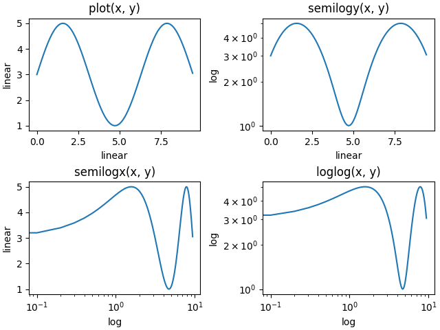
loglog 和 semilogx/y

对数轴的使用非常频繁，因此有一组辅助函数可以实现相同的功能：semilogy、semilogx 和 loglog。

fig, axs = plt.subplot_mosaic([['linear', 'linear-log'],
                               ['log-linear', 'log-log']], layout='constrained')

x = np.arange(0, 3*np.pi, 0.1)
y = 2 * np.sin(x) + 3

ax = axs['linear']
ax.plot(x, y)
ax.set_xlabel('linear')
ax.set_ylabel('linear')
ax.set_title('plot(x, y)')

ax = axs['linear-log']
ax.semilogy(x, y)
ax.set_xlabel('linear')
ax.set_ylabel('log')
ax.set_title('semilogy(x, y)')

ax = axs['log-linear']
ax.semilogx(x, y)
ax.set_xlabel('log')
ax.set_ylabel('linear')
ax.set_title('semilogx(x, y)')

ax = axs['log-log']
ax.loglog(x, y)
ax.set_xlabel('log')
ax.set_ylabel('log')
ax.set_title('loglog(x, y)')

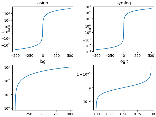
其他内置刻度

还有其他可以使用的刻度。可以从 scale.get_scale_names 返回已注册刻度的列表：

print(mscale.get_scale_names())

['asinh', 'function', 'functionlog', 'linear', 'log', 'logit', 'mercator', 'symlog']

fig, axs = plt.subplot_mosaic([['asinh', 'symlog'],
                               ['log', 'logit']], layout='constrained')

x = np.arange(0, 1000)

for name, ax in axs.items():
    if name in ['asinh', 'symlog']:
        yy = x - np.mean(x)
    elif name in ['logit']:
        yy = (x-np.min(x))
        yy = yy / np.max(np.abs(yy))
    else:
        yy = x

    ax.plot(yy, yy)
    ax.set_yscale(name)
    ax.set_title(name)

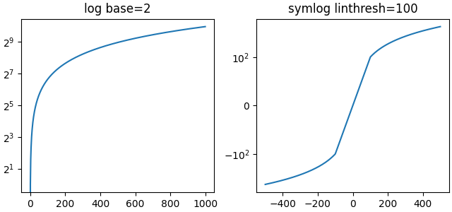
比例的可选参数

一些默认的刻度有可选参数。这些参数在 scale 的 API 参考中有所记录。可以更改绘图中对数的基数（例如下面的 2）或 'symlog' 的线性阈值范围。

fig, axs = plt.subplot_mosaic([['log', 'symlog']], layout='constrained',
                              figsize=(6.4, 3))

for name, ax in axs.items():
    if name in ['log']:
        ax.plot(x, x)
        ax.set_yscale('log', base=2)
        ax.set_title('log base=2')
    else:
        ax.plot(x - np.mean(x), x - np.mean(x))
        ax.set_yscale('symlog', linthresh=100)
        ax.set_title('symlog linthresh=100')

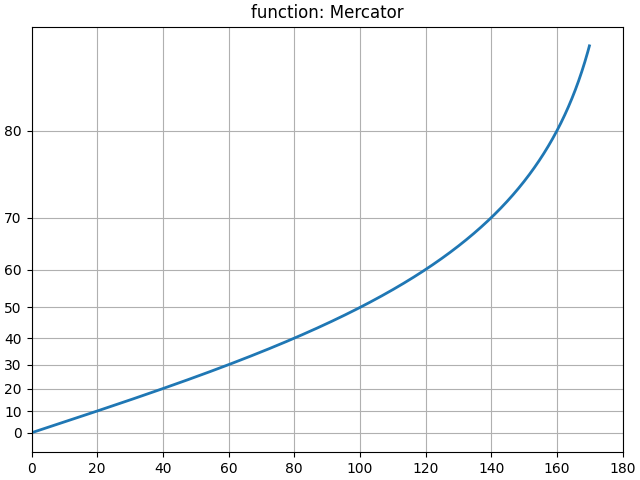
任意函数尺度

用户可以定义一个全尺度的类，并将其传递给 set_xscale 和 set_yscale （参见 自定义比例）。 一个快捷方式是使用 'function' 尺度，并传递额外的参数 forward 和 inverse 函数。 以下代码对 y 轴执行 墨卡托变换。

# Function Mercator transform
def forward(a):
    a = np.deg2rad(a)
    return np.rad2deg(np.log(np.abs(np.tan(a) + 1.0 / np.cos(a))))


def inverse(a):
    a = np.deg2rad(a)
    return np.rad2deg(np.arctan(np.sinh(a)))


t = np.arange(0, 170.0, 0.1)
s = t / 2.

fig, ax = plt.subplots(layout='constrained')
ax.plot(t, s, '-', lw=2)

ax.set_yscale('function', functions=(forward, inverse))
ax.set_title('function: Mercator')
ax.grid(True)
ax.set_xlim([0, 180])
ax.yaxis.set_minor_formatter(NullFormatter())
ax.yaxis.set_major_locator(FixedLocator(np.arange(0, 90, 10)))

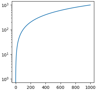
什么是“比例”？

刻度是一个附加到轴上的对象。类文档位于 scale。set_xscale 和 set_yscale 分别设置相应轴对象的刻度。你可以使用 get_scale 来确定轴上的刻度。

fig, ax = plt.subplots(layout='constrained',
                              figsize=(3.2, 3))
ax.semilogy(x, x)

print(ax.xaxis.get_scale())
print(ax.yaxis.get_scale())

linear
log

设置比例会做三件事。首先，它定义了轴上的一个变换，该变换将数据值映射到轴上的位置。这个变换可以通过 get_transform 访问：

print(ax.yaxis.get_transform())

LogTransform(base=10, nonpositive='clip')

轴上的变换是一个相对低级的概念，但它是 set_scale 所扮演的重要角色之一。

设置比例也会设置适合该比例的默认刻度定位器（ticker）和刻度格式化器。具有 'log' 比例的轴使用 LogLocator 在十倍间隔处选择刻度，并使用 LogFormatter 在十倍处使用科学记数法。

print('X axis')
print(ax.xaxis.get_major_locator())
print(ax.xaxis.get_major_formatter())

print('Y axis')
print(ax.yaxis.get_major_locator())
print(ax.yaxis.get_major_formatter())

X axis
<matplotlib.ticker.AutoLocator object at 0x16817e050>
<matplotlib.ticker.ScalarFormatter object at 0x1308a7c90>
Y axis
<matplotlib.ticker.LogLocator object at 0x169b21050>
<matplotlib.ticker.LogFormatterSciNotation object at 0x12c057f10>