约束布局指南

使用 constrained layout 以整洁地适应图表在您的图形中。

Constrained layout 自动调整子图，使得像刻度标签、图例和颜色条这样的装饰不会重叠，同时仍然保留用户请求的逻辑布局。

约束布局 类似于 紧密布局，但更加灵活。它处理放置在多个 Axes 上的颜色条（颜色条放置）、嵌套布局（subfigures）以及跨越行或列的 Axes（subplot_mosaic），力求使同一行或列中的 Axes 的脊线对齐。此外，压缩布局 将尝试将具有固定纵横比的 Axes 移动得更近。这些功能在本文件中进行了描述，以及在最后讨论了一些 实现细节。

约束布局 通常需要在向图形添加任何轴之前激活。有两种方法可以做到这一点。

• 使用 subplots、figure、subplot_mosaic 等各自的参数，例如:

  plt.subplots(layout="constrained")
  

• 通过 rcParams 激活它，例如:

  plt.rcParams['figure.constrained_layout.use'] = True
  

这些内容将在以下章节中详细描述。

警告

调用 tight_layout 将关闭 约束布局！

简单示例

使用默认的坐标轴定位时，坐标轴标题、轴标签或刻度标签有时会超出图形区域，从而被裁剪。

import matplotlib.pyplot as plt
import numpy as np

import matplotlib.colors as mcolors
import matplotlib.gridspec as gridspec

plt.rcParams['savefig.facecolor'] = "0.8"
plt.rcParams['figure.figsize'] = 4.5, 4.
plt.rcParams['figure.max_open_warning'] = 50


def example_plot(ax, fontsize=12, hide_labels=False):
    ax.plot([1, 2])

    ax.locator_params(nbins=3)
    if hide_labels:
        ax.set_xticklabels([])
        ax.set_yticklabels([])
    else:
        ax.set_xlabel('x-label', fontsize=fontsize)
        ax.set_ylabel('y-label', fontsize=fontsize)
        ax.set_title('Title', fontsize=fontsize)

fig, ax = plt.subplots(layout=None)
example_plot(ax, fontsize=24)

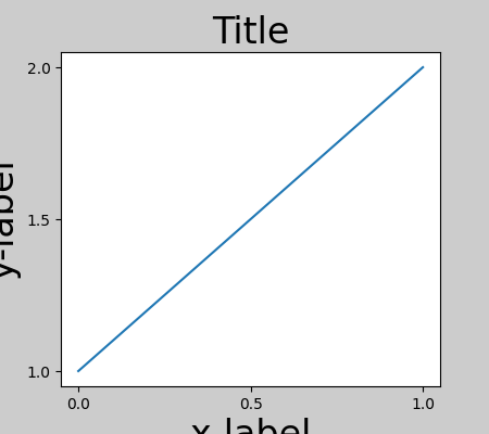
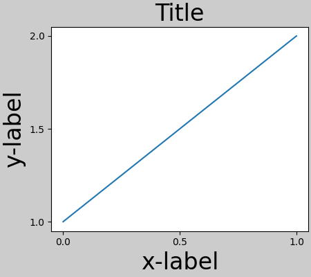
为防止这种情况，需要调整Axes的位置。对于子图，可以通过使用`.Figure.subplots_adjust`手动调整子图参数来实现。然而，通过使用``layout="constrained"``关键字参数指定图形，将自动进行调整。

fig, ax = plt.subplots(layout="constrained")
example_plot(ax, fontsize=24)

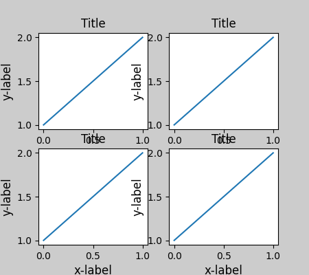
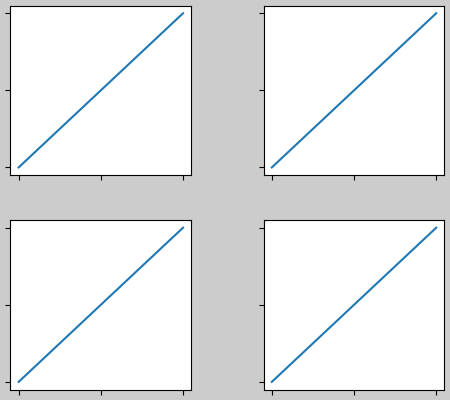
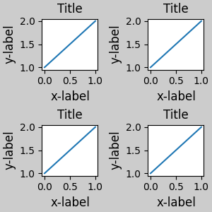
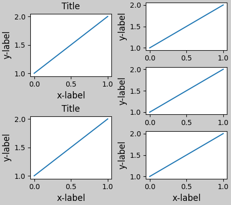
当你有多个子图时，通常你会看到不同 Axes 的标签相互重叠。

fig, axs = plt.subplots(2, 2, layout=None)
for ax in axs.flat:
    example_plot(ax)

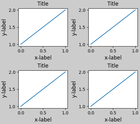
在调用 plt.subplots 时指定 layout="constrained" 会使布局得到适当的约束。

fig, axs = plt.subplots(2, 2, layout="constrained")
for ax in axs.flat:
    example_plot(ax)

颜色条

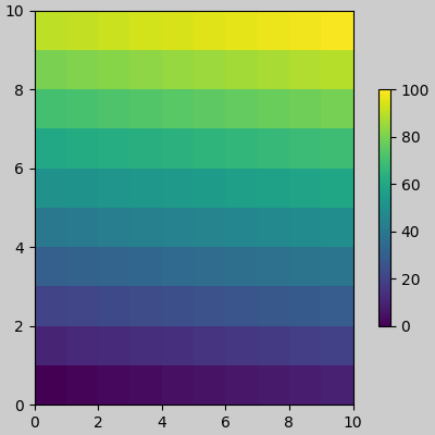
如果你使用 Figure.colorbar 创建一个颜色条，你需要为它腾出空间。约束布局 会自动完成这个任务。注意，如果你指定 use_gridspec=True，它将被忽略，因为这个选项是为了通过 tight_layout 改善布局而设计的。

备注

对于 pcolormesh 的关键字参数 (pc_kwargs)，我们使用字典来保持本文档中的调用一致。

arr = np.arange(100).reshape((10, 10))
norm = mcolors.Normalize(vmin=0., vmax=100.)
# see note above: this makes all pcolormesh calls consistent:
pc_kwargs = {'rasterized': True, 'cmap': 'viridis', 'norm': norm}
fig, ax = plt.subplots(figsize=(4, 4), layout="constrained")
im = ax.pcolormesh(arr, **pc_kwargs)
fig.colorbar(im, ax=ax, shrink=0.6)

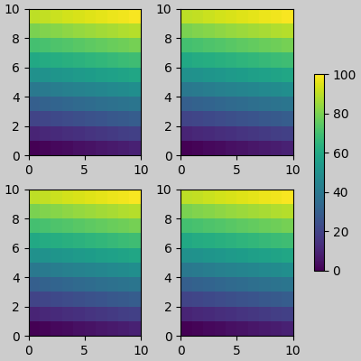
如果你为 colorbar 的 ax 参数指定一个 Axes 列表（或其他可迭代容器），constrained layout 将从指定的 Axes 中获取空间。

fig, axs = plt.subplots(2, 2, figsize=(4, 4), layout="constrained")
for ax in axs.flat:
    im = ax.pcolormesh(arr, **pc_kwargs)
fig.colorbar(im, ax=axs, shrink=0.6)

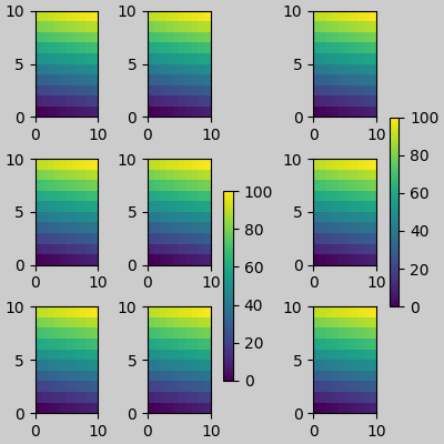
如果你在一个 Axes 网格内部指定一个 Axes 列表，颜色条将适当地占用空间，并留下一个间隙，但所有子图的大小仍将相同。

fig, axs = plt.subplots(3, 3, figsize=(4, 4), layout="constrained")
for ax in axs.flat:
    im = ax.pcolormesh(arr, **pc_kwargs)
fig.colorbar(im, ax=axs[1:, 1], shrink=0.8)
fig.colorbar(im, ax=axs[:, -1], shrink=0.6)

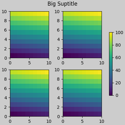
副标题

约束布局 也可以为 suptitle 腾出空间。

fig, axs = plt.subplots(2, 2, figsize=(4, 4), layout="constrained")
for ax in axs.flat:
    im = ax.pcolormesh(arr, **pc_kwargs)
fig.colorbar(im, ax=axs, shrink=0.6)
fig.suptitle('Big Suptitle')

图例

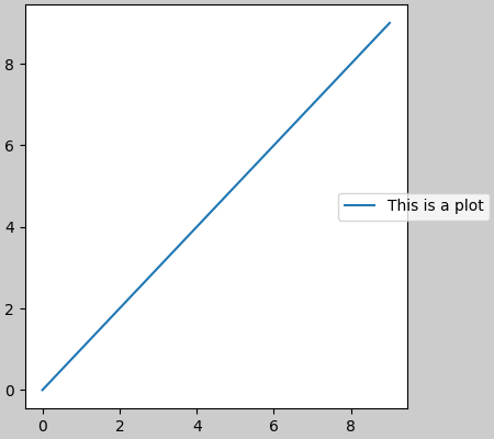
图例可以放置在其父坐标轴之外。约束布局 旨在处理这种情况，适用于 Axes.legend()。然而，约束布局 目前 不 处理通过 Figure.legend() 创建的图例（尚未处理）。

fig, ax = plt.subplots(layout="constrained")
ax.plot(np.arange(10), label='This is a plot')
ax.legend(loc='center left', bbox_to_anchor=(0.8, 0.5))

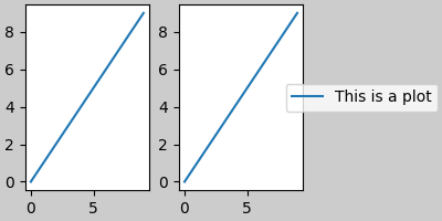
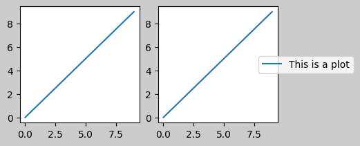
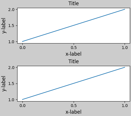
然而，这将从子图布局中占用空间：

fig, axs = plt.subplots(1, 2, figsize=(4, 2), layout="constrained")
axs[0].plot(np.arange(10))
axs[1].plot(np.arange(10), label='This is a plot')
axs[1].legend(loc='center left', bbox_to_anchor=(0.8, 0.5))

为了让图例或其他艺术家*不*从子图布局中占用空间，我们可以 leg.set_in_layout(False)。当然，这可能意味着图例最终会被裁剪，但如果随后使用 fig.savefig('outname.png', bbox_inches='tight') 调用绘图，这可能会很有用。不过请注意，为了使保存的文件正常工作，图例的 get_in_layout 状态需要再次切换，如果我们希望在打印前调整Axes的大小以适应布局，我们必须手动触发绘制。

fig, axs = plt.subplots(1, 2, figsize=(4, 2), layout="constrained")

axs[0].plot(np.arange(10))
axs[1].plot(np.arange(10), label='This is a plot')
leg = axs[1].legend(loc='center left', bbox_to_anchor=(0.8, 0.5))
leg.set_in_layout(False)
# trigger a draw so that constrained layout is executed once
# before we turn it off when printing....
fig.canvas.draw()
# we want the legend included in the bbox_inches='tight' calcs.
leg.set_in_layout(True)
# we don't want the layout to change at this point.
fig.set_layout_engine('none')
try:
    fig.savefig('../../../doc/_static/constrained_layout_1b.png',
                bbox_inches='tight', dpi=100)
except FileNotFoundError:
    # this allows the script to keep going if run interactively and
    # the directory above doesn't exist
    pass

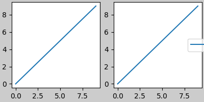
保存的文件看起来像：

解决这种尴尬情况的更好方法是简单地使用 Figure.legend 提供的图例方法：

fig, axs = plt.subplots(1, 2, figsize=(4, 2), layout="constrained")
axs[0].plot(np.arange(10))
lines = axs[1].plot(np.arange(10), label='This is a plot')
labels = [l.get_label() for l in lines]
leg = fig.legend(lines, labels, loc='center left',
                 bbox_to_anchor=(0.8, 0.5), bbox_transform=axs[1].transAxes)
try:
    fig.savefig('../../../doc/_static/constrained_layout_2b.png',
                bbox_inches='tight', dpi=100)
except FileNotFoundError:
    # this allows the script to keep going if run interactively and
    # the directory above doesn't exist
    pass

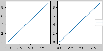
保存的文件看起来像：

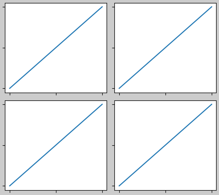
填充和间距

轴之间的填充在水平方向上由 w_pad 和 wspace 控制，在垂直方向上由 h_pad 和 hspace 控制。这些可以通过 set 进行编辑。w/h_pad 是以英寸为单位的轴周围的最小空间：

fig, axs = plt.subplots(2, 2, layout="constrained")
for ax in axs.flat:
    example_plot(ax, hide_labels=True)
fig.get_layout_engine().set(w_pad=4 / 72, h_pad=4 / 72, hspace=0,
                            wspace=0)

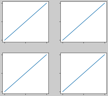
子图之间的间距可以通过 wspace 和 hspace 进一步设置。这些值是作为整个子图组大小的分数来指定的。如果这些值小于 w_pad 或 h_pad，则使用固定的填充。请注意，在下图中，边缘的空间与上图相比没有变化，但子图之间的空间有所不同。

fig, axs = plt.subplots(2, 2, layout="constrained")
for ax in axs.flat:
    example_plot(ax, hide_labels=True)
fig.get_layout_engine().set(w_pad=4 / 72, h_pad=4 / 72, hspace=0.2,
                            wspace=0.2)

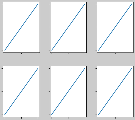
如果有超过两列，wspace 会在它们之间共享，因此这里的 wspace 被分成两部分，每列之间有 0.1 的 wspace：

fig, axs = plt.subplots(2, 3, layout="constrained")
for ax in axs.flat:
    example_plot(ax, hide_labels=True)
fig.get_layout_engine().set(w_pad=4 / 72, h_pad=4 / 72, hspace=0.2,
                            wspace=0.2)

GridSpecs 也有可选的 hspace 和 wspace 关键字参数，这些参数将用于替代 constrained layout 设置的填充。

fig, axs = plt.subplots(2, 2, layout="constrained",
                        gridspec_kw={'wspace': 0.3, 'hspace': 0.2})
for ax in axs.flat:
    example_plot(ax, hide_labels=True)
# this has no effect because the space set in the gridspec trumps the
# space set in *constrained layout*.
fig.get_layout_engine().set(w_pad=4 / 72, h_pad=4 / 72, hspace=0.0,
                            wspace=0.0)

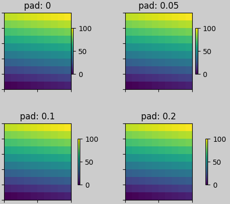
带有颜色条的间距

颜色条与其父对象的距离为 pad ，其中 pad 是父对象宽度的分数。子图之间的间距由 w/hspace 给出。

fig, axs = plt.subplots(2, 2, layout="constrained")
pads = [0, 0.05, 0.1, 0.2]
for pad, ax in zip(pads, axs.flat):
    pc = ax.pcolormesh(arr, **pc_kwargs)
    fig.colorbar(pc, ax=ax, shrink=0.6, pad=pad)
    ax.set_xticklabels([])
    ax.set_yticklabels([])
    ax.set_title(f'pad: {pad}')
fig.get_layout_engine().set(w_pad=2 / 72, h_pad=2 / 72, hspace=0.2,
                            wspace=0.2)

rcParams

有五个 rcParams 可以设置，既可以在脚本中设置，也可以在 matplotlibrc 文件中设置。它们都具有前缀 figure.constrained_layout：

• use: 是否使用 constrained layout。默认是 False

• w_pad, h_pad: 围绕Axes对象的填充。浮点数表示英寸。默认值为3./72.英寸（3磅）

• wspace, hspace: 子图组之间的空间。浮点数表示分离的子图宽度的一部分。默认值为 0.02。

plt.rcParams['figure.constrained_layout.use'] = True
fig, axs = plt.subplots(2, 2, figsize=(3, 3))
for ax in axs.flat:
    example_plot(ax)

与 GridSpec 一起使用

约束布局 旨在与 subplots()、subplot_mosaic() 或 GridSpec() 与 add_subplot() 一起使用。

注意，以下内容中 layout="constrained"

plt.rcParams['figure.constrained_layout.use'] = False
fig = plt.figure(layout="constrained")

gs1 = gridspec.GridSpec(2, 1, figure=fig)
ax1 = fig.add_subplot(gs1[0])
ax2 = fig.add_subplot(gs1[1])

example_plot(ax1)
example_plot(ax2)

更复杂的网格布局是可能的。注意这里我们使用了便捷函数 add_gridspec 和 subgridspec。

fig = plt.figure(layout="constrained")

gs0 = fig.add_gridspec(1, 2)

gs1 = gs0[0].subgridspec(2, 1)
ax1 = fig.add_subplot(gs1[0])
ax2 = fig.add_subplot(gs1[1])

example_plot(ax1)
example_plot(ax2)

gs2 = gs0[1].subgridspec(3, 1)

for ss in gs2:
    ax = fig.add_subplot(ss)
    example_plot(ax)
    ax.set_title("")
    ax.set_xlabel("")

ax.set_xlabel("x-label", fontsize=12)

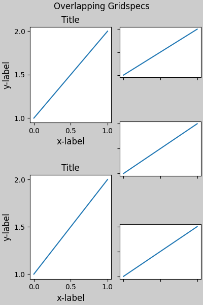
注意，在上面的例子中，左右两列的垂直范围并不相同。如果我们希望两个网格的顶部和底部对齐，那么它们需要在同一个gridspec中。我们还需要使这个图形更大，以便Axes不会缩减为零高度：

fig = plt.figure(figsize=(4, 6), layout="constrained")

gs0 = fig.add_gridspec(6, 2)

ax1 = fig.add_subplot(gs0[:3, 0])
ax2 = fig.add_subplot(gs0[3:, 0])

example_plot(ax1)
example_plot(ax2)

ax = fig.add_subplot(gs0[0:2, 1])
example_plot(ax, hide_labels=True)
ax = fig.add_subplot(gs0[2:4, 1])
example_plot(ax, hide_labels=True)
ax = fig.add_subplot(gs0[4:, 1])
example_plot(ax, hide_labels=True)
fig.suptitle('Overlapping Gridspecs')

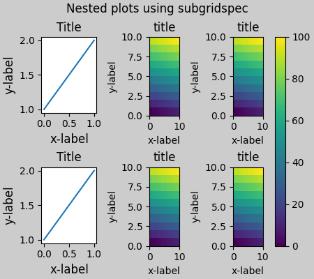
这个例子使用了两个 gridspecs，使得颜色条仅与一组 pcolors 相关。注意左列比右边的两列宽，因为这一点。当然，如果你希望子图大小相同，你只需要一个 gridspec。注意，使用 subfigures 也可以达到同样的效果。

fig = plt.figure(layout="constrained")
gs0 = fig.add_gridspec(1, 2, figure=fig, width_ratios=[1, 2])
gs_left = gs0[0].subgridspec(2, 1)
gs_right = gs0[1].subgridspec(2, 2)

for gs in gs_left:
    ax = fig.add_subplot(gs)
    example_plot(ax)
axs = []
for gs in gs_right:
    ax = fig.add_subplot(gs)
    pcm = ax.pcolormesh(arr, **pc_kwargs)
    ax.set_xlabel('x-label')
    ax.set_ylabel('y-label')
    ax.set_title('title')
    axs += [ax]
fig.suptitle('Nested plots using subgridspec')
fig.colorbar(pcm, ax=axs)

Matplotlib 现在提供了 subfigures，而不是使用子网格规格，这也适用于 约束布局：

fig = plt.figure(layout="constrained")
sfigs = fig.subfigures(1, 2, width_ratios=[1, 2])

axs_left = sfigs[0].subplots(2, 1)
for ax in axs_left.flat:
    example_plot(ax)

axs_right = sfigs[1].subplots(2, 2)
for ax in axs_right.flat:
    pcm = ax.pcolormesh(arr, **pc_kwargs)
    ax.set_xlabel('x-label')
    ax.set_ylabel('y-label')
    ax.set_title('title')
fig.colorbar(pcm, ax=axs_right)
fig.suptitle('Nested plots using subfigures')

手动设置坐标轴位置

手动设置 Axes 位置可能有很好的理由。手动调用 set_position 将设置 Axes，使得 constrained layout 对其不再产生影响。（注意，constrained layout 仍然为移动的 Axes 保留空间）。

fig, axs = plt.subplots(1, 2, layout="constrained")
example_plot(axs[0], fontsize=12)
axs[1].set_position([0.2, 0.2, 0.4, 0.4])

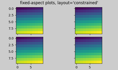
固定纵横比轴的网格：“压缩”布局

约束布局 在 Axes 的“原始”位置网格上操作。然而，当 Axes 具有固定纵横比时，通常会使一边变短，并在缩短的方向上留下较大的间隙。在下面，Axes 是方形的，但图形相当宽，因此在水平方向上有间隙：

fig, axs = plt.subplots(2, 2, figsize=(5, 3),
                        sharex=True, sharey=True, layout="constrained")
for ax in axs.flat:
    ax.imshow(arr)
fig.suptitle("fixed-aspect plots, layout='constrained'")

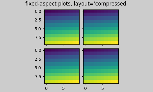
解决这个问题的一个明显方法是使图形尺寸更接近正方形，然而，精确地闭合间隙需要反复试验。对于简单的 Axes 网格，我们可以使用 layout="compressed" 来为我们完成这项工作：

fig, axs = plt.subplots(2, 2, figsize=(5, 3),
                        sharex=True, sharey=True, layout='compressed')
for ax in axs.flat:
    ax.imshow(arr)
fig.suptitle("fixed-aspect plots, layout='compressed'")

手动关闭 constrained layout

约束布局 通常会在每次绘图时调整Axes的位置。如果你想要获得*约束布局*提供的间距，但不希望它更新，那么可以在初始绘图后调用 fig.set_layout_engine('none')。这对于刻度标签长度可能变化的动画可能很有用。

请注意，对于使用工具栏的后端，constrained layout 在 ZOOM 和 PAN GUI 事件中是关闭的。这可以防止在缩放和平移过程中 Axes 的位置发生变化。

限制

不兼容的函数

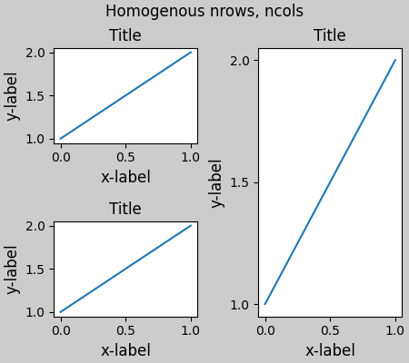
约束布局 将与 pyplot.subplot 一起工作，但前提是每次调用的行数和列数相同。原因是每次调用 pyplot.subplot 时，如果几何形状不同，将创建一个新的 GridSpec 实例，而 约束布局。因此，以下代码可以正常工作：

fig = plt.figure(layout="constrained")

ax1 = plt.subplot(2, 2, 1)
ax2 = plt.subplot(2, 2, 3)
# third Axes that spans both rows in second column:
ax3 = plt.subplot(2, 2, (2, 4))

example_plot(ax1)
example_plot(ax2)
example_plot(ax3)
plt.suptitle('Homogenous nrows, ncols')

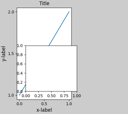
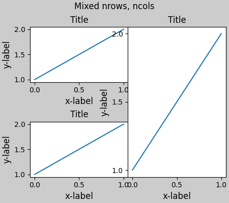
但以下内容会导致布局不佳：

fig = plt.figure(layout="constrained")

ax1 = plt.subplot(2, 2, 1)
ax2 = plt.subplot(2, 2, 3)
ax3 = plt.subplot(1, 2, 2)

example_plot(ax1)
example_plot(ax2)
example_plot(ax3)
plt.suptitle('Mixed nrows, ncols')

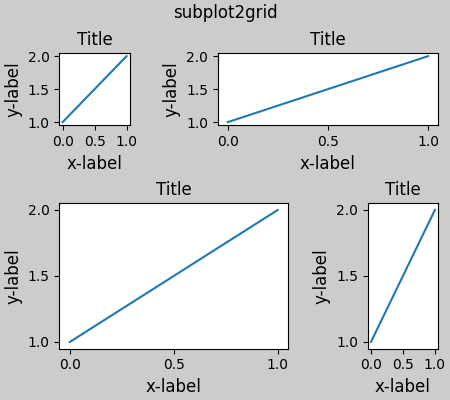
同样地，subplot2grid 也有相同的限制，即 nrows 和 ncols 不能改变，以使布局看起来美观。

fig = plt.figure(layout="constrained")

ax1 = plt.subplot2grid((3, 3), (0, 0))
ax2 = plt.subplot2grid((3, 3), (0, 1), colspan=2)
ax3 = plt.subplot2grid((3, 3), (1, 0), colspan=2, rowspan=2)
ax4 = plt.subplot2grid((3, 3), (1, 2), rowspan=2)

example_plot(ax1)
example_plot(ax2)
example_plot(ax3)
example_plot(ax4)
fig.suptitle('subplot2grid')

其他注意事项

• 受限布局 仅考虑刻度标签、轴标签、标题和图例。因此，其他艺术家可能会被裁剪，也可能重叠。

• 它假设刻度标签、轴标签和标题所需的额外空间与 Axes 的原始位置无关。这通常是正确的，但在极少数情况下并非如此。

• 不同的后端在处理字体渲染时存在细微差异，因此结果不会完全相同。

• 使用超出Axes边界范围的Axes坐标的艺术家在添加到Axes时会导致不寻常的布局。可以通过直接使用 add_artist() 将艺术家添加到 Figure 来避免这种情况。参见 ConnectionPatch 的示例。

调试

约束布局 可能会以一些意想不到的方式失败。因为它使用了一个约束求解器，求解器可能会找到数学上正确但完全不符合用户期望的解决方案。通常的失败模式是所有尺寸都缩小到它们允许的最小值。如果发生这种情况，原因有两个之一：

1. 您请求绘制的元素没有足够的空间。

2. 存在一个错误 - 在这种情况下，请在 matplotlib/matplotlib#issues 打开一个问题。

如果发现错误，请提供一个自包含的示例，该示例不需要外部数据或依赖项（除了numpy）。

算法说明

约束的算法相对简单，但由于我们可以以复杂的方式布局图形，因此具有一定的复杂性。

在 Matplotlib 中，布局是通过 GridSpec 类使用 gridspec 进行的。gridspec 是对图形进行逻辑划分，将其分为行和列，其中 Axes 在这些行和列中的相对宽度由 width_ratios 和 height_ratios 设置。

在 constrained layout 中，每个 gridspec 都会关联一个 layoutgrid。layoutgrid 为每一列设置了 left 和 right 变量，为每一行设置了 bottom 和 top 变量，并且还为左、右、下、上各设置了一个边距。在每一行中，底部/顶部边距会扩大，直到容纳该行中的所有装饰器。类似地，对于列和左/右边距也是如此。

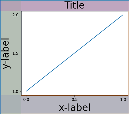
简单情况：一个 Axes

对于单个 Axes 来说，布局是直接的。图表有一个父布局网格，由一行一列组成，还有一个子布局网格用于包含 Axes 的 gridspec，同样由一行一列组成。在 Axes 的每一侧都为“装饰”预留了空间。在代码中，这是通过 do_constrained_layout() 中的条目实现的，例如:

gridspec._layoutgrid[0, 0].edit_margin_min('left',
      -bbox.x0 + pos.x0 + w_pad)

其中 bbox 是 Axes 的紧密边界框，pos 是其位置。注意四个边距如何包围 Axes 的装饰。

from matplotlib._layoutgrid import plot_children

fig, ax = plt.subplots(layout="constrained")
example_plot(ax, fontsize=24)
plot_children(fig)

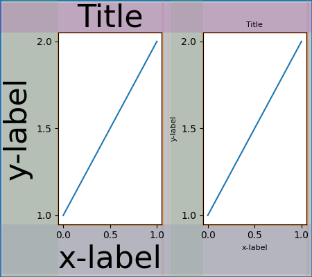
简单情况：两个轴

当有多个 Axes 时，它们的布局以简单的方式绑定。在这个例子中，左边的 Axes 比右边的有更大的装饰，但它们共享一个底部边距，这个边距足够大以容纳更大的 xlabel。同样地，它们也共享顶部边距。左右边距不共享，因此允许不同。

fig, ax = plt.subplots(1, 2, layout="constrained")
example_plot(ax[0], fontsize=32)
example_plot(ax[1], fontsize=8)
plot_children(fig)

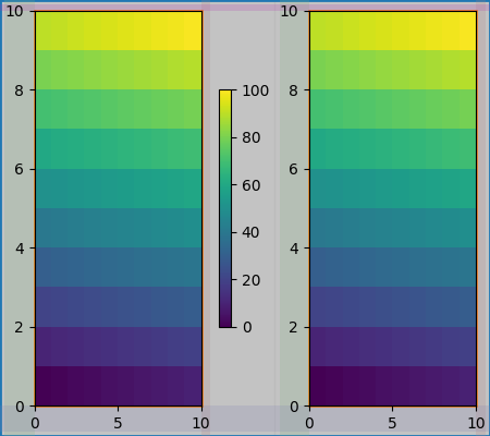
两个坐标轴和颜色条

颜色条只是另一个扩展父布局网格单元格边距的项目：

fig, ax = plt.subplots(1, 2, layout="constrained")
im = ax[0].pcolormesh(arr, **pc_kwargs)
fig.colorbar(im, ax=ax[0], shrink=0.6)
im = ax[1].pcolormesh(arr, **pc_kwargs)
plot_children(fig)

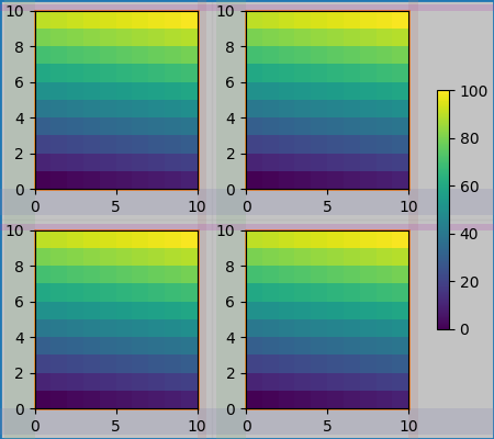
与 Gridspec 关联的颜色条

如果一个颜色条属于网格的多个单元格，那么它会为每个单元格创建一个更大的边距：

fig, axs = plt.subplots(2, 2, layout="constrained")
for ax in axs.flat:
    im = ax.pcolormesh(arr, **pc_kwargs)
fig.colorbar(im, ax=axs, shrink=0.6)
plot_children(fig)

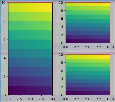
大小不一的坐标轴

在 Gridspec 布局中，有两种方法可以使 Axes 具有不均匀的大小，一种是通过指定它们跨越 Gridspecs 的行或列，另一种是通过指定宽度和高度比率。

第一种方法在这里使用。注意中间的 top 和 bottom 边距不受左侧列的影响。这是算法的有意设计，导致两个右侧的 Axes 具有相同的高度，但它不是左侧 Axes 高度的 1/2。这与 gridspec 在没有 constrained layout 的情况下工作的方式一致。

fig = plt.figure(layout="constrained")
gs = gridspec.GridSpec(2, 2, figure=fig)
ax = fig.add_subplot(gs[:, 0])
im = ax.pcolormesh(arr, **pc_kwargs)
ax = fig.add_subplot(gs[0, 1])
im = ax.pcolormesh(arr, **pc_kwargs)
ax = fig.add_subplot(gs[1, 1])
im = ax.pcolormesh(arr, **pc_kwargs)
plot_children(fig)

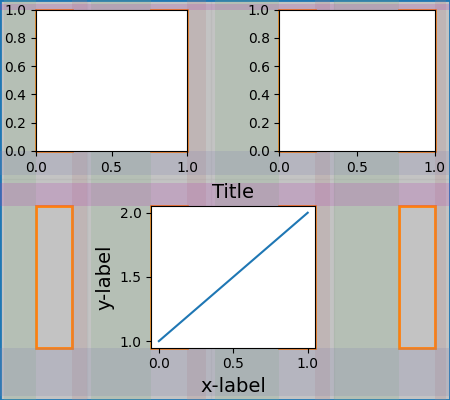
需要微调的一种情况是，如果边距没有任何艺术家限制其宽度。在下面的例子中，第0列的右边距和第3列的左边距没有设置其宽度的边距艺术家，因此我们取那些有艺术家的边距宽度的最大值。这使得所有Axes具有相同的大小：

fig = plt.figure(layout="constrained")
gs = fig.add_gridspec(2, 4)
ax00 = fig.add_subplot(gs[0, 0:2])
ax01 = fig.add_subplot(gs[0, 2:])
ax10 = fig.add_subplot(gs[1, 1:3])
example_plot(ax10, fontsize=14)
plot_children(fig)
plt.show()