复杂且语义化的图形组合 (subplot_mosaic)

在非均匀网格中布置图中的轴既繁琐又冗长。对于密集的均匀网格，我们有 Figure.subplots，但对于更复杂的布局，例如跨越布局中多列/行的轴或留出图的某些区域空白，您可以使用 gridspec.GridSpec`（参见 :ref:`arranging_axes）或手动放置您的轴。Figure.subplot_mosaic 旨在提供一个接口，以视觉方式（无论是ASCII艺术还是嵌套列表）布置您的轴，以简化此过程。

此接口自然支持为您的 Axes 命名。Figure.subplot_mosaic 返回一个以用于布局 Figure 的标签为键的字典。通过返回带有名称的数据结构，编写独立于 Figure 布局的绘图代码变得更加容易。

这是受到 提议的 MEP 和 R 语言的 patchwork 库的启发。虽然我们没有实现操作符重载风格，但我们提供了一个用于指定（嵌套）Axes 布局的 Pythonic API。

import matplotlib.pyplot as plt
import numpy as np


# Helper function used for visualization in the following examples
def identify_axes(ax_dict, fontsize=48):
    """
    Helper to identify the Axes in the examples below.

    Draws the label in a large font in the center of the Axes.

    Parameters
    ----------
    ax_dict : dict[str, Axes]
        Mapping between the title / label and the Axes.
    fontsize : int, optional
        How big the label should be.
    """
    kw = dict(ha="center", va="center", fontsize=fontsize, color="darkgrey")
    for k, ax in ax_dict.items():
        ax.text(0.5, 0.5, k, transform=ax.transAxes, **kw)

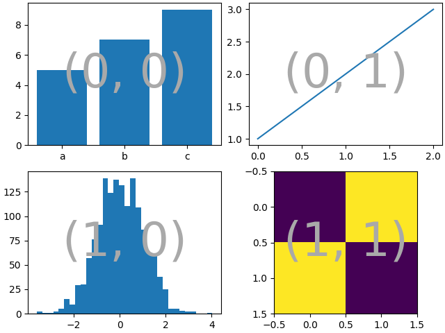
如果我们想要一个2x2的网格，我们可以使用`.Figure.subplots`，它返回一个`.axes.Axes`的二维数组，我们可以对其进行索引以进行绘图。

np.random.seed(19680801)
hist_data = np.random.randn(1_500)


fig = plt.figure(layout="constrained")
ax_array = fig.subplots(2, 2, squeeze=False)

ax_array[0, 0].bar(["a", "b", "c"], [5, 7, 9])
ax_array[0, 1].plot([1, 2, 3])
ax_array[1, 0].hist(hist_data, bins="auto")
ax_array[1, 1].imshow([[1, 2], [2, 1]])

identify_axes(
    {(j, k): a for j, r in enumerate(ax_array) for k, a in enumerate(r)},
)

使用 Figure.subplot_mosaic 我们可以生成相同的马赛克，但给子图赋予语义名称

fig = plt.figure(layout="constrained")
ax_dict = fig.subplot_mosaic(
    [
        ["bar", "plot"],
        ["hist", "image"],
    ],
)
ax_dict["bar"].bar(["a", "b", "c"], [5, 7, 9])
ax_dict["plot"].plot([1, 2, 3])
ax_dict["hist"].hist(hist_data)
ax_dict["image"].imshow([[1, 2], [2, 1]])
identify_axes(ax_dict)

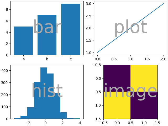
Figure.subplots 和 Figure.subplot_mosaic 之间的一个关键区别在于返回值。前者返回一个用于索引访问的数组，而后者返回一个将标签映射到创建的 axes.Axes 实例的字典。

print(ax_dict)

{'bar': <Axes: label='bar'>, 'plot': <Axes: label='plot'>, 'hist': <Axes: label='hist'>, 'image': <Axes: label='image'>}

字符串简写

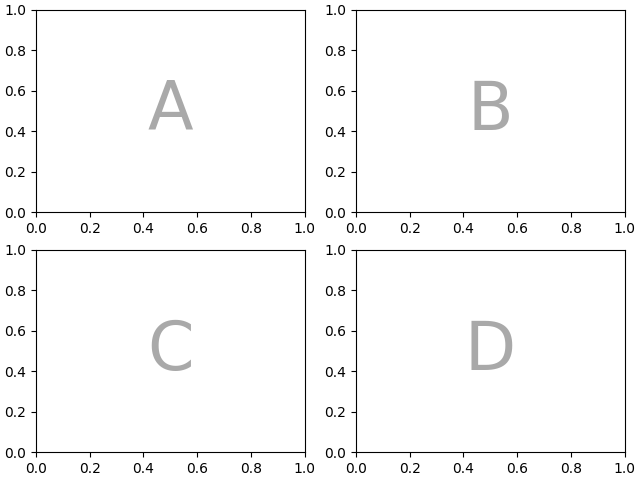
通过将我们的 Axes 标签限制为单个字符，我们可以将我们想要的 Axes “绘制”为“ASCII 艺术”。以下

mosaic = """
    AB
    CD
    """

将为我们提供一个2x2网格布局的4个坐标轴，并生成与上面相同的图形镶嵌（但现在标记为``{"A", "B", "C", "D"}``而不是``{"bar", "plot", "hist", "image"}``）。

fig = plt.figure(layout="constrained")
ax_dict = fig.subplot_mosaic(mosaic)
identify_axes(ax_dict)

或者，您可以使用更紧凑的字符串表示法

mosaic = "AB;CD"

将为您提供相同的组合，其中使用``";"``作为行分隔符，而不是换行符。

fig = plt.figure(layout="constrained")
ax_dict = fig.subplot_mosaic(mosaic)
identify_axes(ax_dict)

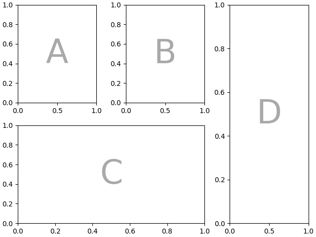
跨越多个行/列的轴

我们可以使用 Figure.subplot_mosaic 做的一件事，而 Figure.subplots 无法做到的是，指定一个 Axes 应该跨越几行或几列。

如果我们想重新排列我们的四个轴，使 "C" 成为底部的水平跨度，而 "D" 成为右侧的垂直跨度，我们会这样做

axd = plt.figure(layout="constrained").subplot_mosaic(
    """
    ABD
    CCD
    """
)
identify_axes(axd)

如果我们不想在图中用 Axes 填充所有空间，我们可以指定网格中的某些空间为空白。

axd = plt.figure(layout="constrained").subplot_mosaic(
    """
    A.C
    BBB
    .D.
    """
)
identify_axes(axd)

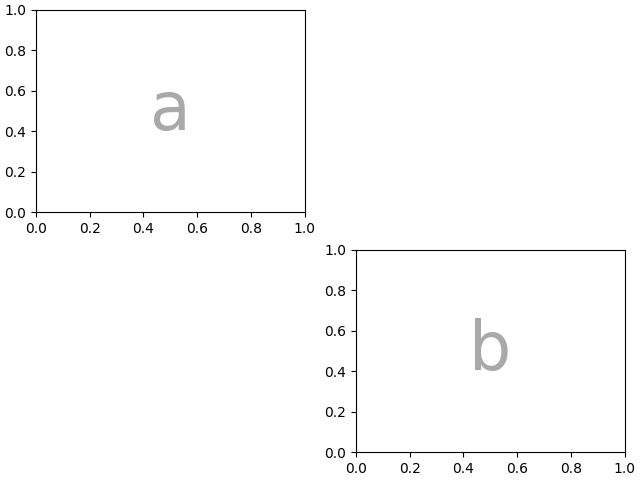
如果我们更倾向于使用另一个字符（而不是句号 "."）来标记空白空间，我们可以使用 empty_sentinel 来指定要使用的字符。

axd = plt.figure(layout="constrained").subplot_mosaic(
    """
    aX
    Xb
    """,
    empty_sentinel="X",
)
identify_axes(axd)

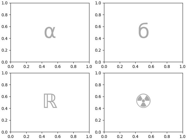
在内部，我们使用的字母没有任何意义，任何Unicode码点都是有效的！

axd = plt.figure(layout="constrained").subplot_mosaic(
    """αб
       ℝ☢"""
)
identify_axes(axd)

不推荐在字符串简写中使用空白作为标签或空占位符，因为在处理输入时可能会被去除。

控制马赛克创建

此功能基于 gridspec 构建，您可以通过关键字参数传递给底层的 gridspec.GridSpec`（与 `.Figure.subplots 相同）。

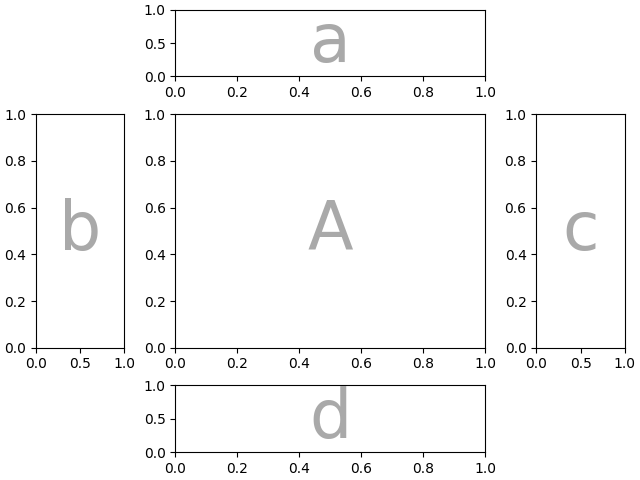
在这种情况下，我们希望使用输入来指定排列，但设置行/列的相对宽度。为了方便，gridspec.GridSpec 的 height_ratios 和 width_ratios 在 Figure.subplot_mosaic 调用序列中暴露出来。

axd = plt.figure(layout="constrained").subplot_mosaic(
    """
    .a.
    bAc
    .d.
    """,
    # set the height ratios between the rows
    height_ratios=[1, 3.5, 1],
    # set the width ratios between the columns
    width_ratios=[1, 3.5, 1],
)
identify_axes(axd)

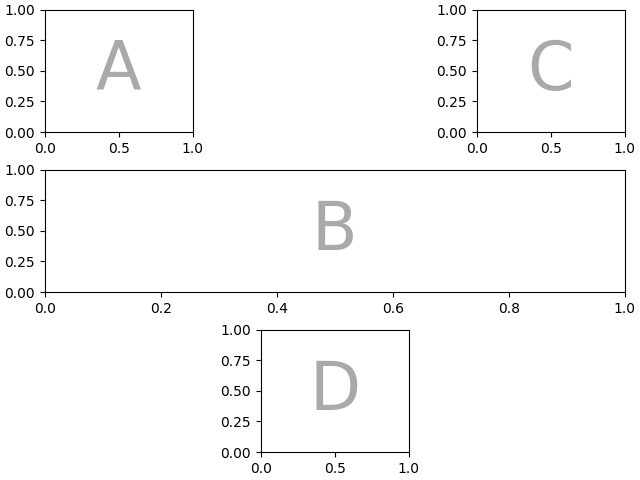
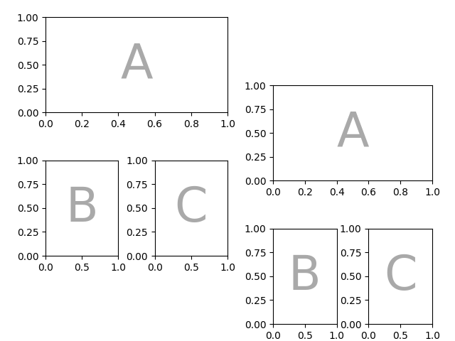
其他 gridspec.GridSpec 关键字可以通过 gridspec_kw 传递。例如，使用 {left, right, bottom, top} 关键字参数来定位整体马赛克，以在图中放置同一马赛克的多个版本。

mosaic = """AA
            BC"""
fig = plt.figure()
axd = fig.subplot_mosaic(
    mosaic,
    gridspec_kw={
        "bottom": 0.25,
        "top": 0.95,
        "left": 0.1,
        "right": 0.5,
        "wspace": 0.5,
        "hspace": 0.5,
    },
)
identify_axes(axd)

axd = fig.subplot_mosaic(
    mosaic,
    gridspec_kw={
        "bottom": 0.05,
        "top": 0.75,
        "left": 0.6,
        "right": 0.95,
        "wspace": 0.5,
        "hspace": 0.5,
    },
)
identify_axes(axd)

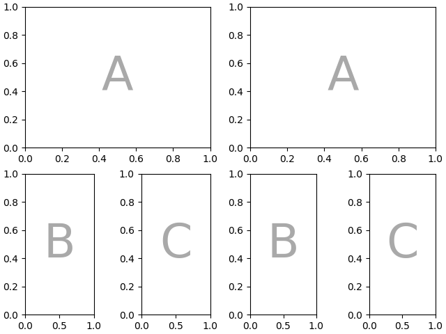
或者，您可以使用子图功能：

mosaic = """AA
            BC"""
fig = plt.figure(layout="constrained")
left, right = fig.subfigures(nrows=1, ncols=2)
axd = left.subplot_mosaic(mosaic)
identify_axes(axd)

axd = right.subplot_mosaic(mosaic)
identify_axes(axd)

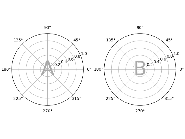
控制子图创建

我们还可以传递用于创建子图的参数（同样，与 Figure.subplots 相同），这些参数将应用于所有创建的 Axes。

axd = plt.figure(layout="constrained").subplot_mosaic(
    "AB", subplot_kw={"projection": "polar"}
)
identify_axes(axd)

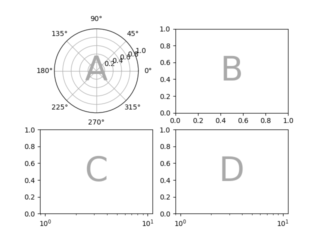
每个轴的子图关键字参数

如果你需要单独控制传递给每个子图的参数，使用 per_subplot_kw 来传递一个映射，该映射将 Axes 标识符（或 Axes 标识符的元组）映射到要传递的关键字字典。

Added in version 3.7.

fig, axd = plt.subplot_mosaic(
    "AB;CD",
    per_subplot_kw={
        "A": {"projection": "polar"},
        ("C", "D"): {"xscale": "log"}
    },
)
identify_axes(axd)

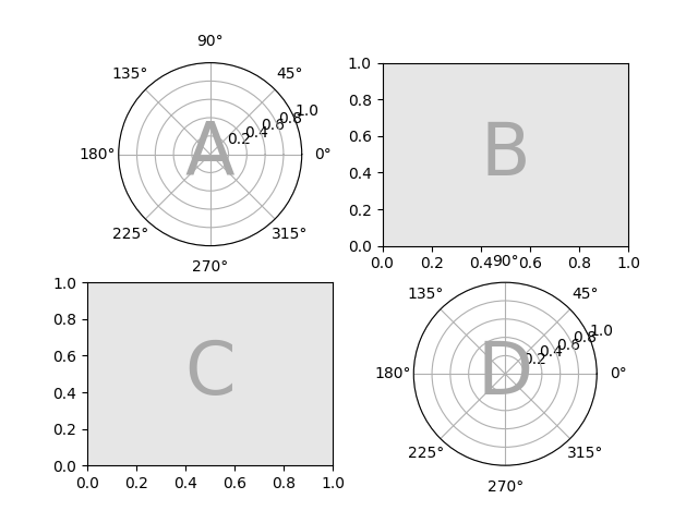
如果布局是用字符串简写指定的，那么我们知道轴标签将是一个字符，并且可以明确地解释 per_subplot_kw 中的较长字符串，以指定一组轴来应用关键字：

fig, axd = plt.subplot_mosaic(
    "AB;CD",
    per_subplot_kw={
        "AD": {"projection": "polar"},
        "BC": {"facecolor": ".9"}
    },
)
identify_axes(axd)

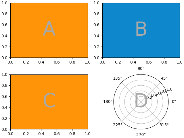
如果同时使用 subplot_kw 和 per_subplot_kw ，则它们会合并，优先使用 per_subplot_kw ：

axd = plt.figure(layout="constrained").subplot_mosaic(
    "AB;CD",
    subplot_kw={"facecolor": "xkcd:tangerine"},
    per_subplot_kw={
        "B": {"facecolor": "xkcd:water blue"},
        "D": {"projection": "polar", "facecolor": "w"},
    }
)
identify_axes(axd)

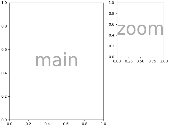
嵌套列表输入

我们可以使用字符串简写形式做的所有事情，也可以在传递列表时完成（内部我们将字符串简写形式转换为嵌套列表），例如使用跨度、空白和 gridspec_kw：

axd = plt.figure(layout="constrained").subplot_mosaic(
    [
        ["main", "zoom"],
        ["main", "BLANK"],
    ],
    empty_sentinel="BLANK",
    width_ratios=[2, 1],
)
identify_axes(axd)

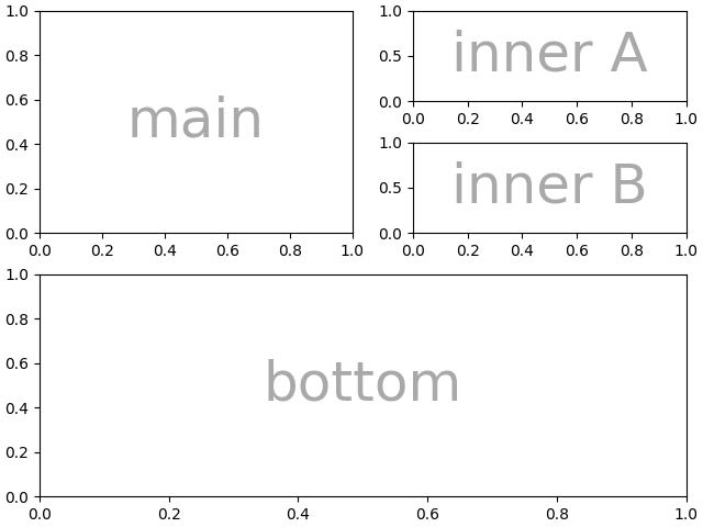
此外，使用列表输入，我们可以指定嵌套的马赛克。内部列表的任何元素都可以是另一组嵌套列表：

inner = [
    ["inner A"],
    ["inner B"],
]

outer_nested_mosaic = [
    ["main", inner],
    ["bottom", "bottom"],
]
axd = plt.figure(layout="constrained").subplot_mosaic(
    outer_nested_mosaic, empty_sentinel=None
)
identify_axes(axd, fontsize=36)

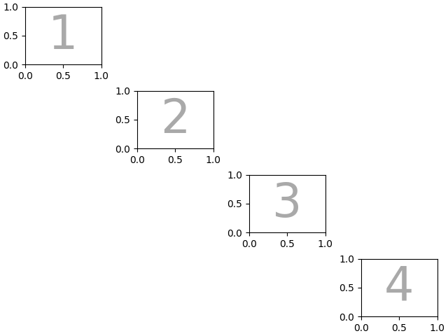
我们也可以传入一个二维的 NumPy 数组来执行诸如

mosaic = np.zeros((4, 4), dtype=int)
for j in range(4):
    mosaic[j, j] = j + 1
axd = plt.figure(layout="constrained").subplot_mosaic(
    mosaic,
    empty_sentinel=0,
)
identify_axes(axd)