备注
前往结尾 下载完整示例代码。
绘制日期和字符串#
使用 Matplotlib 绘图方法的最基本方式是将坐标作为数值 numpy 数组传递。例如,如果 x 和 y 是浮点数(或整数)的 numpy 数组,则 plot(x, y) 将有效。如果 numpy.asarray 可以将 x 和 y 转换为浮点数数组,绘图方法也将有效;例如,x 可以是 python 列表。
Matplotlib 还具有转换其他数据类型的能力,如果该数据类型存在“单位转换器”。Matplotlib 内置了两个转换器,一个用于日期,另一个用于字符串列表。其他下游库有自己的转换器来处理它们的数据类型。
在 matplotlib.units 中描述了向 Matplotlib 添加转换器的方法。这里我们简要概述内置的日期和字符串转换器。
日期转换#
如果 x 和/或 y 是 datetime 列表或 numpy.datetime64 数组,Matplotlib 有一个内置的转换器,可以将日期时间转换为浮点数,并为轴添加适合日期的刻度定位器和格式化器。参见 matplotlib.dates。
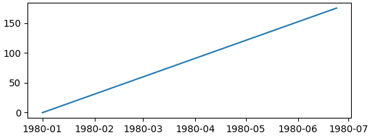
在下面的例子中,x轴获得了一个转换器,该转换器将 numpy.datetime64 转换为浮点数,以及一个在月初放置刻度的定位器,和一个适当地标记刻度的格式化器:
import numpy as np

import matplotlib.dates as mdates
import matplotlib.units as munits

import matplotlib.pyplot as plt

fig, ax = plt.subplots(figsize=(5.4, 2), layout='constrained')
time = np.arange('1980-01-01', '1980-06-25', dtype='datetime64[D]')
x = np.arange(len(time))
ax.plot(time, x)
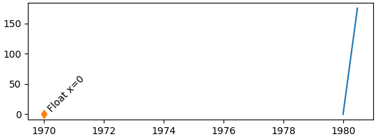
请注意,如果我们尝试在x轴上绘制一个浮点数,它将以转换器“纪元”以来的天数为单位进行绘制,在本例中为1970-01-01(参见 日期格式)。因此,当我们绘制值0时,刻度从1970-01-01开始。(定位器现在选择每两年为一个刻度,而不是每个月):
fig, ax = plt.subplots(figsize=(5.4, 2), layout='constrained')
time = np.arange('1980-01-01', '1980-06-25', dtype='datetime64[D]')
x = np.arange(len(time))
ax.plot(time, x)
# 0 gets labeled as 1970-01-01
ax.plot(0, 0, 'd')
ax.text(0, 0, ' Float x=0', rotation=45)
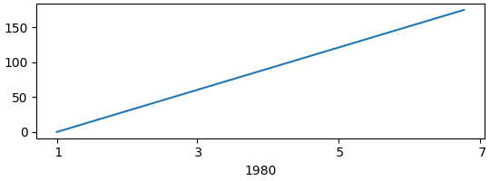
我们可以自定义定位器和格式化器;参见 日期刻度定位器 和 日期格式化器 以获取完整列表,以及 日期刻度定位器和格式化器 以查看使用示例。这里我们按每两个月定位一次,并使用 "%b" 仅格式化为月份的3个字母名称(参见 strftime 以获取格式代码):
fig, ax = plt.subplots(figsize=(5.4, 2), layout='constrained')
time = np.arange('1980-01-01', '1980-06-25', dtype='datetime64[D]')
x = np.arange(len(time))
ax.plot(time, x)
ax.xaxis.set_major_locator(mdates.MonthLocator(bymonth=np.arange(1, 13, 2)))
ax.xaxis.set_major_formatter(mdates.DateFormatter('%b'))
ax.set_xlabel('1980')
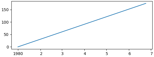
默认的定位器是 AutoDateLocator,默认的格式化器是 AutoDateFormatter。还有“简洁”的格式化器和定位器,它们提供更紧凑的标签,可以通过 rcParams 设置。注意,与年初冗余的“Jan”标签不同,这里使用了“1980”。更多示例请参见 使用 ConciseDateFormatter 格式化日期刻度。
plt.rcParams['date.converter'] = 'concise'

fig, ax = plt.subplots(figsize=(5.4, 2), layout='constrained')
time = np.arange('1980-01-01', '1980-06-25', dtype='datetime64[D]')
x = np.arange(len(time))
ax.plot(time, x)
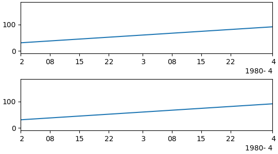
我们可以通过传递适当的日期作为限制,或者通过传递自纪元以来的适当单位的浮点值来设置轴的限制。如果需要,我们可以从 date2num 获取此值。
fig, axs = plt.subplots(2, 1, figsize=(5.4, 3), layout='constrained')
for ax in axs.flat:
    time = np.arange('1980-01-01', '1980-06-25', dtype='datetime64[D]')
    x = np.arange(len(time))
    ax.plot(time, x)

# set xlim using datetime64:
axs[0].set_xlim(np.datetime64('1980-02-01'), np.datetime64('1980-04-01'))

# set xlim using floats:
# Note can get from mdates.date2num(np.datetime64('1980-02-01'))
axs[1].set_xlim(3683, 3683+60)
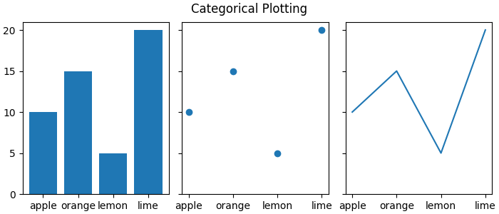
字符串转换:分类图#
有时我们希望在轴上标注类别而不是数字。Matplotlib 允许使用“分类”转换器来实现这一点(参见 category)。
data = {'apple': 10, 'orange': 15, 'lemon': 5, 'lime': 20}
names = list(data.keys())
values = list(data.values())

fig, axs = plt.subplots(1, 3, figsize=(7, 3), sharey=True, layout='constrained')
axs[0].bar(names, values)
axs[1].scatter(names, values)
axs[2].plot(names, values)
fig.suptitle('Categorical Plotting')
请注意,“类别”是按照它们首次指定的顺序绘制的,并且后续以不同顺序绘制不会影响原始顺序。此外,新添加的内容将被添加到末尾(见下文的“pear”):
fig, ax = plt.subplots(figsize=(5, 3), layout='constrained')
ax.bar(names, values)

# plot in a different order:
ax.scatter(['lemon', 'apple'], [7, 12])

# add a new category, "pear", and put the other categories in a different order:
ax.plot(['pear', 'orange', 'apple', 'lemon'], [13, 10, 7, 12], color='C1')
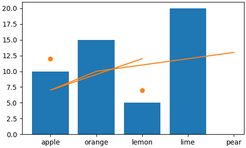
请注意,当像上面那样使用 plot 时,绘图的顺序会映射到数据的原始顺序,因此新行会按照指定的顺序排列。
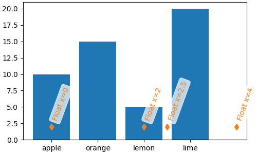
类别转换器将类别映射为从零开始的整数。因此,数据也可以使用浮点数手动添加到轴上。请注意,如果传入的浮点数没有与之关联的“类别”,数据点仍然可以绘制,但不会在那里创建刻度。在下面,我们在4.0和2.5处绘制数据,但由于这些不是类别,因此不会在那里添加刻度。
fig, ax = plt.subplots(figsize=(5, 3), layout='constrained')
ax.bar(names, values)
# arguments for styling the labels below:
args = {'rotation': 70, 'color': 'C1',
        'bbox': {'color': 'white', 'alpha': .7, 'boxstyle': 'round'}}


# 0 gets labeled as "apple"
ax.plot(0, 2, 'd', color='C1')
ax.text(0, 3, 'Float x=0', **args)

# 2 gets labeled as "lemon"
ax.plot(2, 2, 'd', color='C1')
ax.text(2, 3, 'Float x=2', **args)

# 4 doesn't get a label
ax.plot(4, 2, 'd', color='C1')
ax.text(4, 3, 'Float x=4', **args)

# 2.5 doesn't get a label
ax.plot(2.5, 2, 'd', color='C1')
ax.text(2.5, 3, 'Float x=2.5', **args)
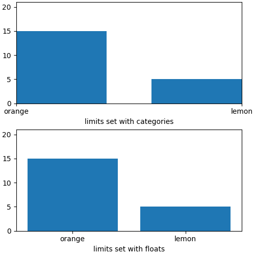
设置类别轴的限制可以通过指定类别或通过指定浮点数来完成:
fig, axs = plt.subplots(2, 1, figsize=(5, 5), layout='constrained')
ax = axs[0]
ax.bar(names, values)
ax.set_xlim('orange', 'lemon')
ax.set_xlabel('limits set with categories')
ax = axs[1]
ax.bar(names, values)
ax.set_xlim(0.5, 2.5)
ax.set_xlabel('limits set with floats')
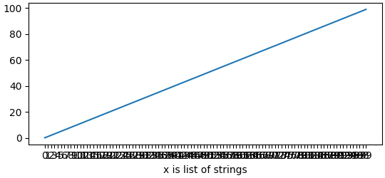
类别轴对于某些绘图类型很有帮助,但如果数据被读取为字符串列表,即使它本应是浮点数或日期的列表,也可能导致混淆。这种情况有时发生在读取逗号分隔值(CSV)文件时。类别定位器和格式化器将在每个字符串值处放置一个刻度,并为每个值添加标签:
fig, ax = plt.subplots(figsize=(5.4, 2.5), layout='constrained')
x = [str(xx) for xx in np.arange(100)]  # list of strings
ax.plot(x, np.arange(100))
ax.set_xlabel('x is list of strings')
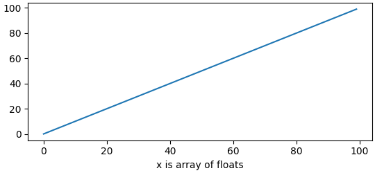
如果这不是期望的,那么在绘图之前简单地将数据转换为浮点数:
fig, ax = plt.subplots(figsize=(5.4, 2.5), layout='constrained')
x = np.asarray(x, dtype='float')  # array of float.
ax.plot(x, np.arange(100))
ax.set_xlabel('x is array of floats')
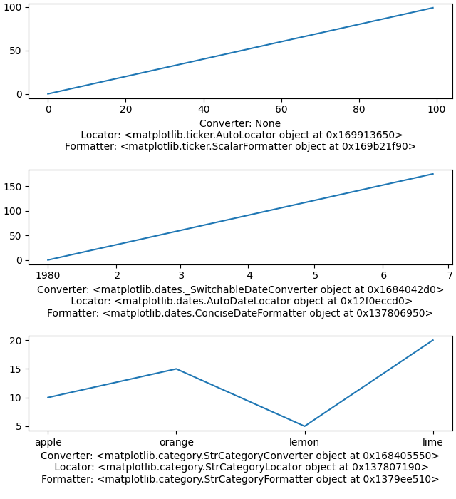
确定轴上的转换器、格式化器和定位器#
有时,能够调试 Matplotlib 用于转换传入数据的工具是很有帮助的。我们可以通过查询轴上的 converter 属性来实现这一点。我们还可以使用 get_major_locator 和 get_major_formatter 来查询格式化器和定位器。
请注意,默认情况下转换器是 None。
fig, axs = plt.subplots(3, 1, figsize=(6.4, 7), layout='constrained')
x = np.arange(100)
ax = axs[0]
ax.plot(x, x)
label = f'Converter: {ax.xaxis.converter}\n '
label += f'Locator: {ax.xaxis.get_major_locator()}\n'
label += f'Formatter: {ax.xaxis.get_major_formatter()}\n'
ax.set_xlabel(label)

ax = axs[1]
time = np.arange('1980-01-01', '1980-06-25', dtype='datetime64[D]')
x = np.arange(len(time))
ax.plot(time, x)
label = f'Converter: {ax.xaxis.converter}\n '
label += f'Locator: {ax.xaxis.get_major_locator()}\n'
label += f'Formatter: {ax.xaxis.get_major_formatter()}\n'
ax.set_xlabel(label)

ax = axs[2]
data = {'apple': 10, 'orange': 15, 'lemon': 5, 'lime': 20}
names = list(data.keys())
values = list(data.values())
ax.plot(names, values)
label = f'Converter: {ax.xaxis.converter}\n '
label += f'Locator: {ax.xaxis.get_major_locator()}\n'
label += f'Formatter: {ax.xaxis.get_major_formatter()}\n'
ax.set_xlabel(label)
更多关于“单元”支持的内容#
对日期和类别的支持是 Matplotlib 内置的“单位”支持的一部分。这在 matplotlib.units 中描述,并在 基本单位 示例中进行了说明。
单位支持通过查询传递给绘图函数的数据类型,并将其分派到接受该数据类型的转换器列表中的第一个转换器来工作。因此,在下面,如果 x 包含 datetime 对象,转换器将是 _SwitchableDateConverter;如果它包含字符串,它将被发送到 StrCategoryConverter。
for k, v in munits.registry.items():
    print(f"type: {k};\n    converter: {type(v)}")
type: <class 'decimal.Decimal'>;
    converter: <class 'matplotlib.units.DecimalConverter'>
type: <class 'numpy.datetime64'>;
    converter: <class 'matplotlib.dates._SwitchableDateConverter'>
type: <class 'datetime.date'>;
    converter: <class 'matplotlib.dates._SwitchableDateConverter'>
type: <class 'datetime.datetime'>;
    converter: <class 'matplotlib.dates._SwitchableDateConverter'>
type: <class 'str'>;
    converter: <class 'matplotlib.category.StrCategoryConverter'>
type: <class 'numpy.str_'>;
    converter: <class 'matplotlib.category.StrCategoryConverter'>
type: <class 'bytes'>;
    converter: <class 'matplotlib.category.StrCategoryConverter'>
type: <class 'numpy.bytes_'>;
    converter: <class 'matplotlib.category.StrCategoryConverter'>
有许多下游库提供了带有定位器和格式化器的转换器。物理单位支持由 astropy、pint 和 unyt 等提供。
像 pandas 和 nc-time-axis <https://nc-time-axis.readthedocs.io>`_(因此也包括 `xarray)这样的高级库提供了它们自己的日期时间支持。这种支持有时可能与 Matplotlib 原生的日期时间支持不兼容,因此在使用这些库时,如果使用 Matplotlib 的定位器和格式化器,应格外小心。
脚本总运行时间: (0 分钟 1.511 秒)