注意
跳转到末尾 以下载完整示例代码。
使用Python进行最优传输介绍
本示例介绍了如何在Python中使用最优运输。
# Author: Remi Flamary, Nicolas Courty, Aurelie Boisbunon
#
# License: MIT License
# sphinx_gallery_thumbnail_number = 1
POT Python 最优传输工具箱
POT 安装
使用 pip 安装:
pip install pot
使用 conda 安装:
conda install -c conda-forge pot
导入工具箱
import numpy as np  # always need it
import pylab as pl  # do the plots

import ot  # ot

import time
获取帮助
在线文档 : https://pythonot.github.io/all.html
或者在线帮助:
help(ot.dist)
Help on function dist in module ot.utils:

dist(x1, x2=None, metric='sqeuclidean', p=2, w=None)
    Compute distance between samples in :math:`\mathbf{x_1}` and :math:`\mathbf{x_2}`

    .. note:: This function is backend-compatible and will work on arrays
        from all compatible backends.

    Parameters
    ----------

    x1 : array-like, shape (n1,d)
        matrix with `n1` samples of size `d`
    x2 : array-like, shape (n2,d), optional
        matrix with `n2` samples of size `d` (if None then :math:`\mathbf{x_2} = \mathbf{x_1}`)
    metric : str | callable, optional
        'sqeuclidean' or 'euclidean' on all backends. On numpy the function also
        accepts  from the scipy.spatial.distance.cdist function : 'braycurtis',
        'canberra', 'chebyshev', 'cityblock', 'correlation', 'cosine', 'dice',
        'euclidean', 'hamming', 'jaccard', 'kulczynski1', 'mahalanobis',
        'matching', 'minkowski', 'rogerstanimoto', 'russellrao', 'seuclidean',
        'sokalmichener', 'sokalsneath', 'sqeuclidean', 'wminkowski', 'yule'.
    p : float, optional
        p-norm for the Minkowski and the Weighted Minkowski metrics. Default value is 2.
    w : array-like, rank 1
        Weights for the weighted metrics.


    Returns
    -------

    M : array-like, shape (`n1`, `n2`)
        distance matrix computed with given metric
第一个 OT 问题
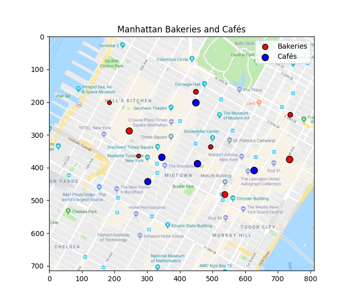
我们将解决面包店/咖啡厅的问题,将羊角面包从多个面包店运送到城市中的咖啡厅(在这种情况下是曼哈顿)。我们在曼哈顿快速搜索了面包店和咖啡厅:

我们从这个搜索中提取了它们的位置,并生成了虚构的生产和销售数字(两者总和相同)。
我们可以获取面包店的位置信息 bakery_pos 及其
各自的生产量 bakery_prod,这些信息描述了源分布。出售羊角面包的咖啡馆也通过
它们的位置 cafe_pos 和 cafe_prod 定义,并描述目标
分布。为了好玩,我们还提供一个
地图 Imap,将展示这些商店在城市中的位置。
现在我们加载数据
data = np.load("../data/manhattan.npz")

bakery_pos = data["bakery_pos"]
bakery_prod = data["bakery_prod"]
cafe_pos = data["cafe_pos"]
cafe_prod = data["cafe_prod"]
Imap = data["Imap"]

print("Bakery production: {}".format(bakery_prod))
print("Cafe sale: {}".format(cafe_prod))
print("Total croissants : {}".format(cafe_prod.sum()))
Bakery production: [31. 48. 82. 30. 40. 48. 89. 73.]
Cafe sale: [82. 88. 92. 88. 91.]
Total croissants : 441.0
在城市中绘制面包店
接下来我们在地图上绘制面包店和咖啡馆的位置。圆圈的大小与它们的产量成正比。
pl.figure(1, (7, 6))
pl.clf()
pl.imshow(Imap, interpolation="bilinear")  # plot the map
pl.scatter(
    bakery_pos[:, 0], bakery_pos[:, 1], s=bakery_prod, c="r", ec="k", label="Bakeries"
)
pl.scatter(cafe_pos[:, 0], cafe_pos[:, 1], s=cafe_prod, c="b", ec="k", label="Cafés")
pl.legend()
pl.title("Manhattan Bakeries and Cafés")
Text(0.5, 1.0, 'Manhattan Bakeries and Cafés')
成本矩阵
我们现在可以计算面包店和咖啡馆之间的成本矩阵,这将是运输成本矩阵。这可以使用ot.dist函数完成,该函数默认使用平方欧几里得距离,但也可以返回其他内容,例如城市块距离(或曼哈顿距离)。
C = ot.dist(bakery_pos, cafe_pos)

labels = [str(i) for i in range(len(bakery_prod))]
f = pl.figure(2, (14, 7))
pl.clf()
pl.subplot(121)
pl.imshow(Imap, interpolation="bilinear")  # plot the map
for i in range(len(cafe_pos)):
    pl.text(
        cafe_pos[i, 0],
        cafe_pos[i, 1],
        labels[i],
        color="b",
        fontsize=14,
        fontweight="bold",
        ha="center",
        va="center",
    )
for i in range(len(bakery_pos)):
    pl.text(
        bakery_pos[i, 0],
        bakery_pos[i, 1],
        labels[i],
        color="r",
        fontsize=14,
        fontweight="bold",
        ha="center",
        va="center",
    )
pl.title("Manhattan Bakeries and Cafés")

ax = pl.subplot(122)
im = pl.imshow(C, cmap="coolwarm")
pl.title("Cost matrix")
cbar = pl.colorbar(im, ax=ax, shrink=0.5, use_gridspec=True)
cbar.ax.set_ylabel("cost", rotation=-90, va="bottom")

pl.xlabel("Cafés")
pl.ylabel("Bakeries")
pl.tight_layout()
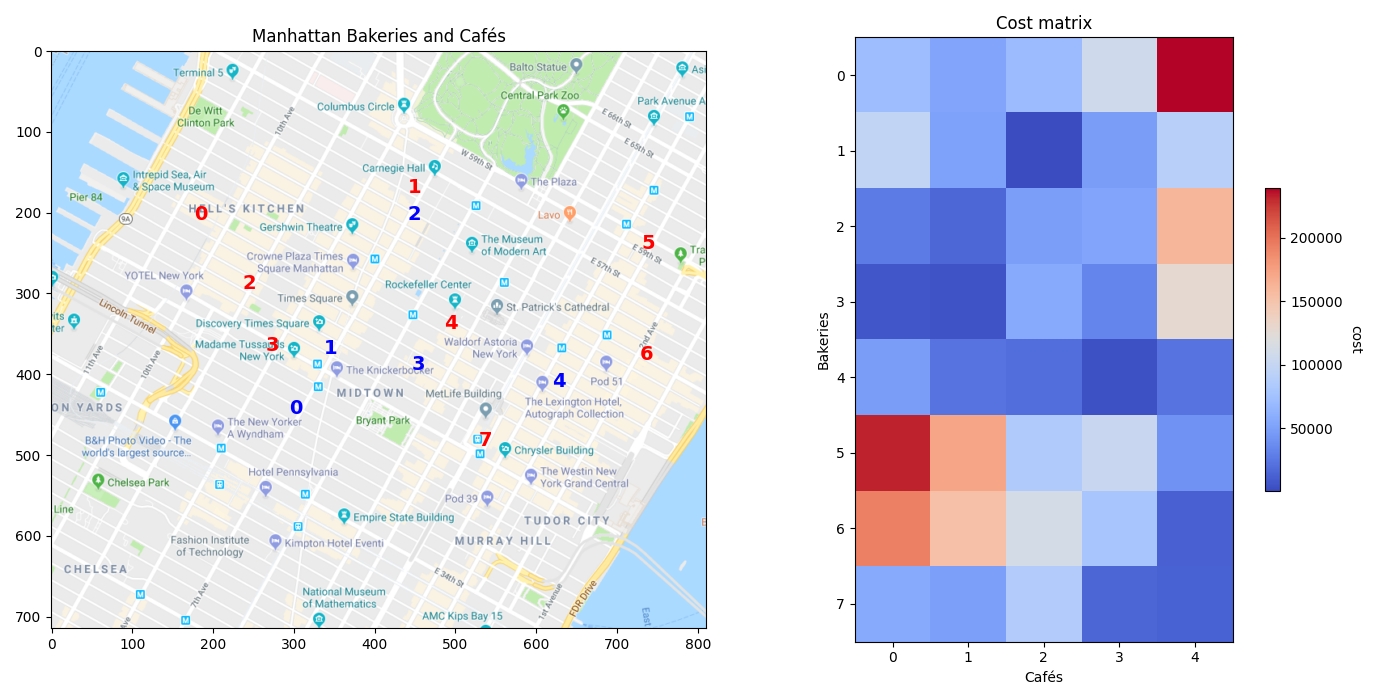
矩阵图像中的红色单元格显示的是离得较远的面包店和咖啡馆,因此从一个运输到另一个的成本更高,而蓝色单元格显示的是相互之间非常接近的面包店和咖啡馆,相对于平方欧几里得距离。
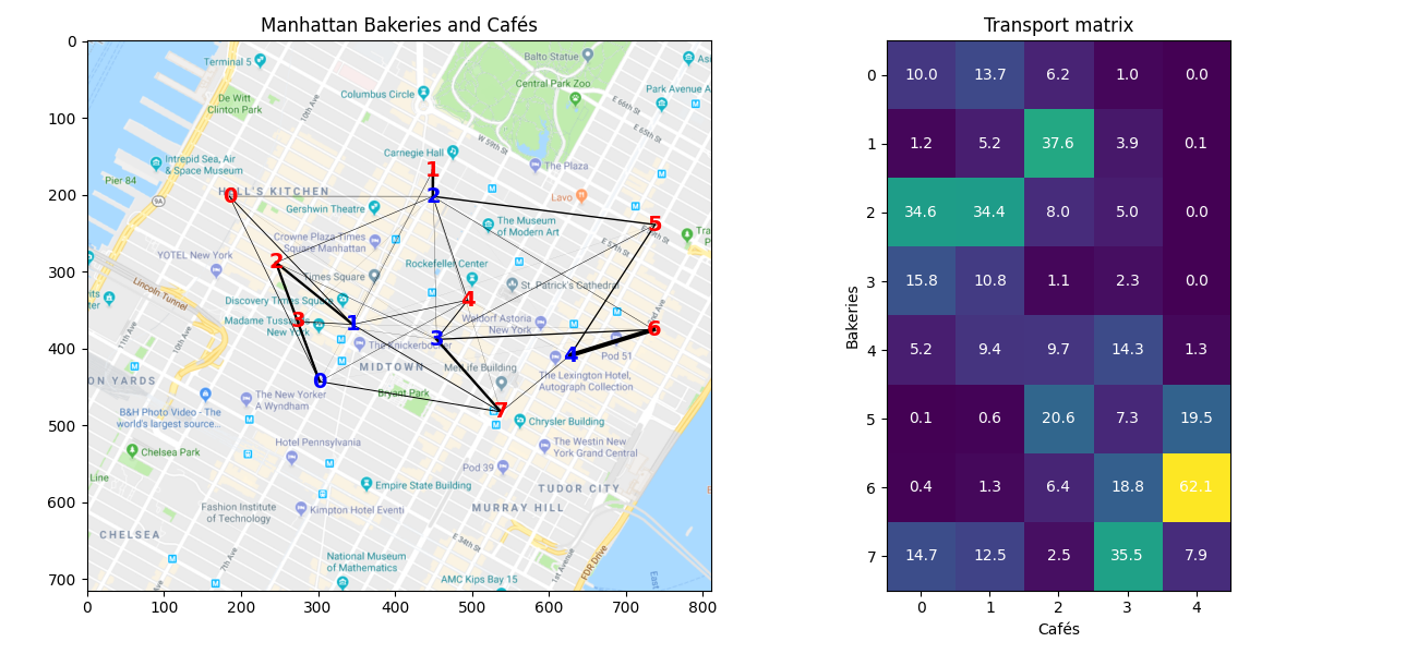
使用 ot.emd 解决OT问题
该函数返回传输矩阵,我们可以在下一个部分进行可视化。
交通计划可视化
在二维平面中对OT矩阵进行良好的可视化就是用一条线表示面包店和咖啡馆之间的质量运输。这可以通过一个双for循环轻松实现。
为了使其更具可解释性,可以使用 alpha 参数并将其设置为 alpha=G[i,j]/G.max()。
# Plot the matrix and the map
f = pl.figure(3, (14, 7))
pl.clf()
pl.subplot(121)
pl.imshow(Imap, interpolation="bilinear")  # plot the map
for i in range(len(bakery_pos)):
    for j in range(len(cafe_pos)):
        pl.plot(
            [bakery_pos[i, 0], cafe_pos[j, 0]],
            [bakery_pos[i, 1], cafe_pos[j, 1]],
            "-k",
            lw=3.0 * ot_emd[i, j] / ot_emd.max(),
        )
for i in range(len(cafe_pos)):
    pl.text(
        cafe_pos[i, 0],
        cafe_pos[i, 1],
        labels[i],
        color="b",
        fontsize=14,
        fontweight="bold",
        ha="center",
        va="center",
    )
for i in range(len(bakery_pos)):
    pl.text(
        bakery_pos[i, 0],
        bakery_pos[i, 1],
        labels[i],
        color="r",
        fontsize=14,
        fontweight="bold",
        ha="center",
        va="center",
    )
pl.title("Manhattan Bakeries and Cafés")

ax = pl.subplot(122)
im = pl.imshow(ot_emd)
for i in range(len(bakery_prod)):
    for j in range(len(cafe_prod)):
        text = ax.text(
            j, i, "{0:g}".format(ot_emd[i, j]), ha="center", va="center", color="w"
        )
pl.title("Transport matrix")

pl.xlabel("Cafés")
pl.ylabel("Bakeries")
pl.tight_layout()

运输矩阵给出了每个面包店可以运输到每个咖啡馆的可颂数量。我们可以看到,面包店只需要将可颂运输到一个或两个咖啡馆,运输矩阵非常稀疏。
OT损失及对偶变量
得到的Wasserstein损失形式为:
其中 \(\gamma\) 是最优传输矩阵。
Wasserstein loss (EMD) = 10838179.41
带有Sinkhorn的正则化OT
Sinkhorn算法的编码非常简单。您可以使用以下伪代码直接实现它
在这个算法中,\(\oslash\) 对应于元素级除法。
另一种选择是使用POT工具箱中的 ot.sinkhorn
注意数值问题。对Sinkhorn来说,一种好的预处理方法是将成本矩阵 C 除以它的最大值。
算法
# Compute Sinkhorn transport matrix from algorithm
reg = 0.1
K = np.exp(-C / C.max() / reg)
nit = 100
u = np.ones((len(bakery_prod),))
for i in range(1, nit):
    v = cafe_prod / np.dot(K.T, u)
    u = bakery_prod / (np.dot(K, v))
ot_sink_algo = np.atleast_2d(u).T * (
    K * v.T
)  # Equivalent to np.dot(np.diag(u), np.dot(K, np.diag(v)))

# Compute Sinkhorn transport matrix with POT
ot_sinkhorn = ot.sinkhorn(bakery_prod, cafe_prod, reg=reg, M=C / C.max())

# Difference between the 2
print(
    "Difference between algo and ot.sinkhorn = {0:.2g}".format(
        np.sum(np.power(ot_sink_algo - ot_sinkhorn, 2))
    )
)
Difference between algo and ot.sinkhorn = 2.1e-20
绘制矩阵和地图
print("Min. of Sinkhorn's transport matrix = {0:.2g}".format(np.min(ot_sinkhorn)))

f = pl.figure(4, (13, 6))
pl.clf()
pl.subplot(121)
pl.imshow(Imap, interpolation="bilinear")  # plot the map
for i in range(len(bakery_pos)):
    for j in range(len(cafe_pos)):
        pl.plot(
            [bakery_pos[i, 0], cafe_pos[j, 0]],
            [bakery_pos[i, 1], cafe_pos[j, 1]],
            "-k",
            lw=3.0 * ot_sinkhorn[i, j] / ot_sinkhorn.max(),
        )
for i in range(len(cafe_pos)):
    pl.text(
        cafe_pos[i, 0],
        cafe_pos[i, 1],
        labels[i],
        color="b",
        fontsize=14,
        fontweight="bold",
        ha="center",
        va="center",
    )
for i in range(len(bakery_pos)):
    pl.text(
        bakery_pos[i, 0],
        bakery_pos[i, 1],
        labels[i],
        color="r",
        fontsize=14,
        fontweight="bold",
        ha="center",
        va="center",
    )
pl.title("Manhattan Bakeries and Cafés")

ax = pl.subplot(122)
im = pl.imshow(ot_sinkhorn)
for i in range(len(bakery_prod)):
    for j in range(len(cafe_prod)):
        text = ax.text(
            j, i, np.round(ot_sinkhorn[i, j], 1), ha="center", va="center", color="w"
        )
pl.title("Transport matrix")

pl.xlabel("Cafés")
pl.ylabel("Bakeries")
pl.tight_layout()
Min. of Sinkhorn's transport matrix = 0.0008
我们马上注意到,使用Sinkhorn方法时矩阵并不是稀疏的,每个面包店都将可颂送到所有5家咖啡馆。此外,这种解决方案产生的运输量是分数,这在可颂的情况下没有意义。这在EMD方法中并不是这样的。
在Sinkhorn中变化正则化参数
reg_parameter = np.logspace(-3, 0, 20)
W_sinkhorn_reg = np.zeros((len(reg_parameter),))
time_sinkhorn_reg = np.zeros((len(reg_parameter),))

f = pl.figure(5, (14, 5))
pl.clf()
max_ot = 100  # plot matrices with the same colorbar
for k in range(len(reg_parameter)):
    start = time.time()
    ot_sinkhorn = ot.sinkhorn(
        bakery_prod, cafe_prod, reg=reg_parameter[k], M=C / C.max()
    )
    time_sinkhorn_reg[k] = time.time() - start

    if k % 4 == 0 and k > 0:  # we only plot a few
        ax = pl.subplot(1, 5, k // 4)
        im = pl.imshow(ot_sinkhorn, vmin=0, vmax=max_ot)
        pl.title("reg={0:.2g}".format(reg_parameter[k]))
        pl.xlabel("Cafés")
        pl.ylabel("Bakeries")

    # Compute the Wasserstein loss for Sinkhorn, and compare with EMD
    W_sinkhorn_reg[k] = np.sum(ot_sinkhorn * C)
pl.tight_layout()
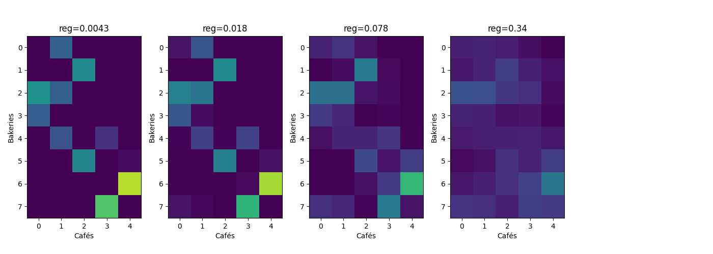
/home/circleci/project/ot/bregman/_sinkhorn.py:667: UserWarning: Sinkhorn did not converge. You might want to increase the number of iterations `numItermax` or the regularization parameter `reg`.
  warnings.warn(
这一系列图表显示,Sinkhorn的解在正则化参数非常小的情况下开始时与EMD非常相似(尽管不是稀疏的),并且随着正则化参数的增加趋向于更均匀的解。
瓦瑟斯坦损失和计算时间
# Plot the matrix and the map
f = pl.figure(6, (4, 4))
pl.clf()
pl.title("Comparison between Sinkhorn and EMD")

pl.plot(reg_parameter, W_sinkhorn_reg, "o", label="Sinkhorn")
XLim = pl.xlim()
pl.plot(XLim, [W, W], "--k", label="EMD")
pl.legend()
pl.xlabel("reg")
pl.ylabel("Wasserstein loss")
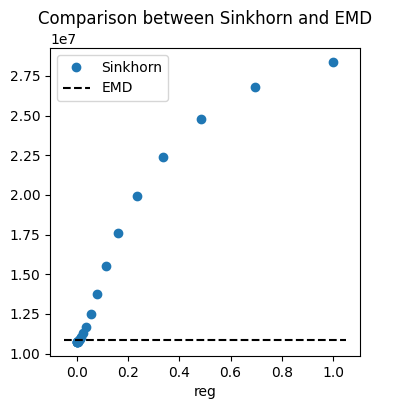
Text(3.972222222222223, 0.5, 'Wasserstein loss')
在最后的这张图中,我们展示了正则化参数对Wasserstein损失的影响。我们可以看到,更高的reg值会导致Wasserstein损失显著增加。
EMD的Wasserstein损失被展示以供比较。对于低值的 reg,Sinkhorn的Wasserstein损失可能会低一点,但它很快会变得高得多。
脚本的总运行时间: (0分钟 2.140秒)