使用不同的地面度量的最优传输

具有不同基础度量的经验分布上的二维OT。

从https://arxiv.org/pdf/1706.07650.pdf中的图1和图2窃取了图形创意

# Author: Remi Flamary <remi.flamary@unice.fr>
#
# License: MIT License

# sphinx_gallery_thumbnail_number = 3

import numpy as np
import matplotlib.pylab as pl
import ot
import ot.plot

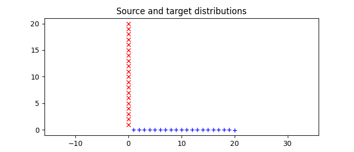
数据集 1 : 均匀抽样

n = 20  # nb samples
xs = np.zeros((n, 2))
xs[:, 0] = np.arange(n) + 1
xs[:, 1] = (np.arange(n) + 1) * -0.001  # to make it strictly convex...

xt = np.zeros((n, 2))
xt[:, 1] = np.arange(n) + 1

a, b = ot.unif(n), ot.unif(n)  # uniform distribution on samples

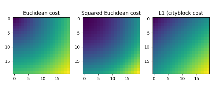
# loss matrix
M1 = ot.dist(xs, xt, metric="euclidean")
M1 /= M1.max()

# loss matrix
M2 = ot.dist(xs, xt, metric="sqeuclidean")
M2 /= M2.max()

# loss matrix
Mp = ot.dist(xs, xt, metric="cityblock")
Mp /= Mp.max()

# Data
pl.figure(1, figsize=(7, 3))
pl.clf()
pl.plot(xs[:, 0], xs[:, 1], "+b", label="Source samples")
pl.plot(xt[:, 0], xt[:, 1], "xr", label="Target samples")
pl.axis("equal")
pl.title("Source and target distributions")


# Cost matrices
pl.figure(2, figsize=(7, 3))

pl.subplot(1, 3, 1)
pl.imshow(M1, interpolation="nearest")
pl.title("Euclidean cost")

pl.subplot(1, 3, 2)
pl.imshow(M2, interpolation="nearest")
pl.title("Squared Euclidean cost")

pl.subplot(1, 3, 3)
pl.imshow(Mp, interpolation="nearest")
pl.title("L1 (cityblock cost")
pl.tight_layout()

• 
• 

数据集 1 : 绘制 OT 矩阵

G1 = ot.emd(a, b, M1)
G2 = ot.emd(a, b, M2)
Gp = ot.emd(a, b, Mp)

# OT matrices
pl.figure(3, figsize=(7, 3))

pl.subplot(1, 3, 1)
ot.plot.plot2D_samples_mat(xs, xt, G1, c=[0.5, 0.5, 1])
pl.plot(xs[:, 0], xs[:, 1], "+b", label="Source samples")
pl.plot(xt[:, 0], xt[:, 1], "xr", label="Target samples")
pl.axis("equal")
# pl.legend(loc=0)
pl.title("OT Euclidean")

pl.subplot(1, 3, 2)
ot.plot.plot2D_samples_mat(xs, xt, G2, c=[0.5, 0.5, 1])
pl.plot(xs[:, 0], xs[:, 1], "+b", label="Source samples")
pl.plot(xt[:, 0], xt[:, 1], "xr", label="Target samples")
pl.axis("equal")
# pl.legend(loc=0)
pl.title("OT squared Euclidean")

pl.subplot(1, 3, 3)
ot.plot.plot2D_samples_mat(xs, xt, Gp, c=[0.5, 0.5, 1])
pl.plot(xs[:, 0], xs[:, 1], "+b", label="Source samples")
pl.plot(xt[:, 0], xt[:, 1], "xr", label="Target samples")
pl.axis("equal")
# pl.legend(loc=0)
pl.title("OT L1 (cityblock)")
pl.tight_layout()

pl.show()

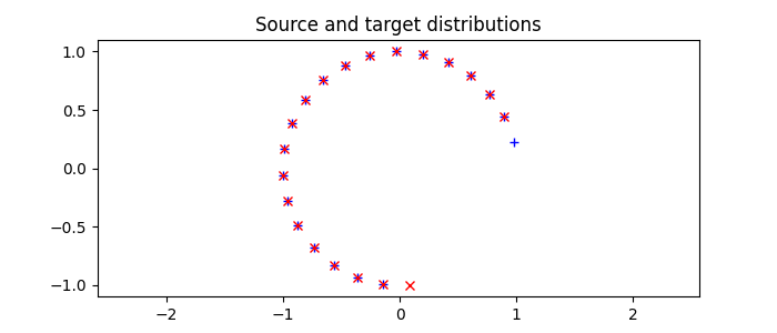
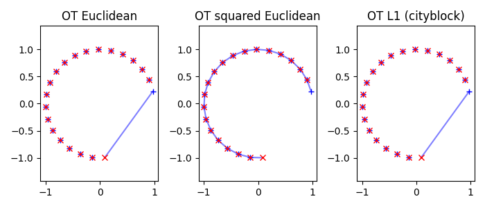
数据集 2 : 部分圆

n = 20  # nb samples
xtot = np.zeros((n + 1, 2))
xtot[:, 0] = np.cos((np.arange(n + 1) + 1.0) * 0.8 / (n + 2) * 2 * np.pi)
xtot[:, 1] = np.sin((np.arange(n + 1) + 1.0) * 0.8 / (n + 2) * 2 * np.pi)

xs = xtot[:n, :]
xt = xtot[1:, :]

a, b = ot.unif(n), ot.unif(n)  # uniform distribution on samples

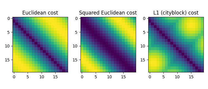
# loss matrix
M1 = ot.dist(xs, xt, metric="euclidean")
M1 /= M1.max()

# loss matrix
M2 = ot.dist(xs, xt, metric="sqeuclidean")
M2 /= M2.max()

# loss matrix
Mp = ot.dist(xs, xt, metric="cityblock")
Mp /= Mp.max()


# Data
pl.figure(4, figsize=(7, 3))
pl.clf()
pl.plot(xs[:, 0], xs[:, 1], "+b", label="Source samples")
pl.plot(xt[:, 0], xt[:, 1], "xr", label="Target samples")
pl.axis("equal")
pl.title("Source and target distributions")


# Cost matrices
pl.figure(5, figsize=(7, 3))

pl.subplot(1, 3, 1)
pl.imshow(M1, interpolation="nearest")
pl.title("Euclidean cost")

pl.subplot(1, 3, 2)
pl.imshow(M2, interpolation="nearest")
pl.title("Squared Euclidean cost")

pl.subplot(1, 3, 3)
pl.imshow(Mp, interpolation="nearest")
pl.title("L1 (cityblock) cost")
pl.tight_layout()

• 
• 

数据集 2 : 绘制 OT 矩阵

G1 = ot.emd(a, b, M1)
G2 = ot.emd(a, b, M2)
Gp = ot.emd(a, b, Mp)

# OT matrices
pl.figure(6, figsize=(7, 3))

pl.subplot(1, 3, 1)
ot.plot.plot2D_samples_mat(xs, xt, G1, c=[0.5, 0.5, 1])
pl.plot(xs[:, 0], xs[:, 1], "+b", label="Source samples")
pl.plot(xt[:, 0], xt[:, 1], "xr", label="Target samples")
pl.axis("equal")
# pl.legend(loc=0)
pl.title("OT Euclidean")

pl.subplot(1, 3, 2)
ot.plot.plot2D_samples_mat(xs, xt, G2, c=[0.5, 0.5, 1])
pl.plot(xs[:, 0], xs[:, 1], "+b", label="Source samples")
pl.plot(xt[:, 0], xt[:, 1], "xr", label="Target samples")
pl.axis("equal")
# pl.legend(loc=0)
pl.title("OT squared Euclidean")

pl.subplot(1, 3, 3)
ot.plot.plot2D_samples_mat(xs, xt, Gp, c=[0.5, 0.5, 1])
pl.plot(xs[:, 0], xs[:, 1], "+b", label="Source samples")
pl.plot(xt[:, 0], xt[:, 1], "xr", label="Target samples")
pl.axis("equal")
# pl.legend(loc=0)
pl.title("OT L1 (cityblock)")
pl.tight_layout()

pl.show()