二维经验分布之间的最优传输

在分布之间进行2D最优运输的示意图，这些分布是Diracs的加权和。OT矩阵与样本一起绘制。

# Author: Remi Flamary <remi.flamary@unice.fr>
#         Kilian Fatras <kilian.fatras@irisa.fr>
#
# License: MIT License

# sphinx_gallery_thumbnail_number = 4

import numpy as np
import matplotlib.pylab as pl
import ot
import ot.plot

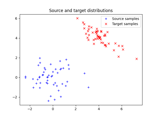
生成数据

n = 50  # nb samples

mu_s = np.array([0, 0])
cov_s = np.array([[1, 0], [0, 1]])

mu_t = np.array([4, 4])
cov_t = np.array([[1, -0.8], [-0.8, 1]])

xs = ot.datasets.make_2D_samples_gauss(n, mu_s, cov_s)
xt = ot.datasets.make_2D_samples_gauss(n, mu_t, cov_t)

a, b = np.ones((n,)) / n, np.ones((n,)) / n  # uniform distribution on samples

# loss matrix
M = ot.dist(xs, xt)

绘制数据

pl.figure(1)
pl.plot(xs[:, 0], xs[:, 1], "+b", label="Source samples")
pl.plot(xt[:, 0], xt[:, 1], "xr", label="Target samples")
pl.legend(loc=0)
pl.title("Source and target distributions")

pl.figure(2)
pl.imshow(M, interpolation="nearest")
pl.title("Cost matrix M")

• 
• 

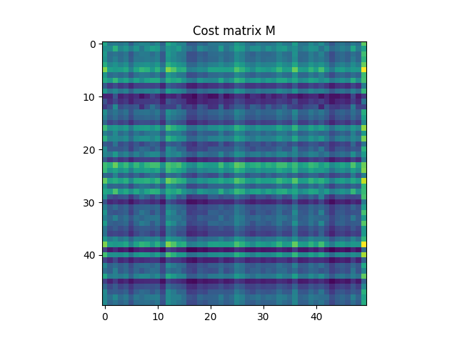
Text(0.5, 1.0, 'Cost matrix M')

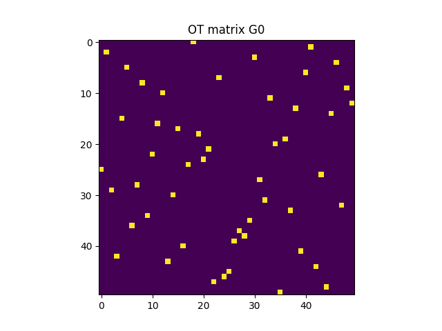
计算EMD

G0 = ot.emd(a, b, M)

pl.figure(3)
pl.imshow(G0, interpolation="nearest")
pl.title("OT matrix G0")

pl.figure(4)
ot.plot.plot2D_samples_mat(xs, xt, G0, c=[0.5, 0.5, 1])
pl.plot(xs[:, 0], xs[:, 1], "+b", label="Source samples")
pl.plot(xt[:, 0], xt[:, 1], "xr", label="Target samples")
pl.legend(loc=0)
pl.title("OT matrix with samples")

• 
• 

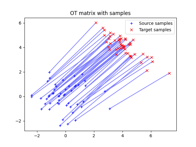
Text(0.5, 1.0, 'OT matrix with samples')

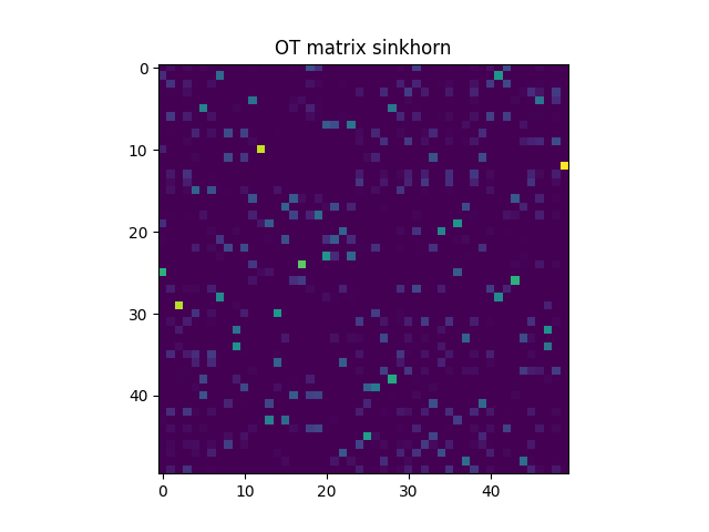
计算Sinkhorn

# reg term
lambd = 1e-1

Gs = ot.sinkhorn(a, b, M, lambd)

pl.figure(5)
pl.imshow(Gs, interpolation="nearest")
pl.title("OT matrix sinkhorn")

pl.figure(6)
ot.plot.plot2D_samples_mat(xs, xt, Gs, color=[0.5, 0.5, 1])
pl.plot(xs[:, 0], xs[:, 1], "+b", label="Source samples")
pl.plot(xt[:, 0], xt[:, 1], "xr", label="Target samples")
pl.legend(loc=0)
pl.title("OT matrix Sinkhorn with samples")

pl.show()

• 
• 

/home/circleci/project/ot/bregman/_sinkhorn.py:667: UserWarning: Sinkhorn did not converge. You might want to increase the number of iterations `numItermax` or the regularization parameter `reg`.
  warnings.warn(

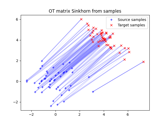
经验Sinkhorn

# reg term
lambd = 1e-1

Ges = ot.bregman.empirical_sinkhorn(xs, xt, lambd)

pl.figure(7)
pl.imshow(Ges, interpolation="nearest")
pl.title("OT matrix empirical sinkhorn")

pl.figure(8)
ot.plot.plot2D_samples_mat(xs, xt, Ges, color=[0.5, 0.5, 1])
pl.plot(xs[:, 0], xs[:, 1], "+b", label="Source samples")
pl.plot(xt[:, 0], xt[:, 1], "xr", label="Target samples")
pl.legend(loc=0)
pl.title("OT matrix Sinkhorn from samples")

pl.show()

• 
•