一维分布的最优运输

这个例子展示了EMD和Sinkhorn传输计划的计算及其可视化。

# Author: Remi Flamary <remi.flamary@unice.fr>
#
# License: MIT License
# sphinx_gallery_thumbnail_number = 3

import numpy as np
import matplotlib.pylab as pl
import ot
import ot.plot
from ot.datasets import make_1D_gauss as gauss

生成数据

n = 100  # nb bins

# bin positions
x = np.arange(n, dtype=np.float64)

# Gaussian distributions
a = gauss(n, m=20, s=5)  # m= mean, s= std
b = gauss(n, m=60, s=10)

# loss matrix
M = ot.dist(x.reshape((n, 1)), x.reshape((n, 1)))
M /= M.max()

绘制分布和损失矩阵

pl.figure(1, figsize=(6.4, 3))
pl.plot(x, a, "b", label="Source distribution")
pl.plot(x, b, "r", label="Target distribution")
pl.legend()

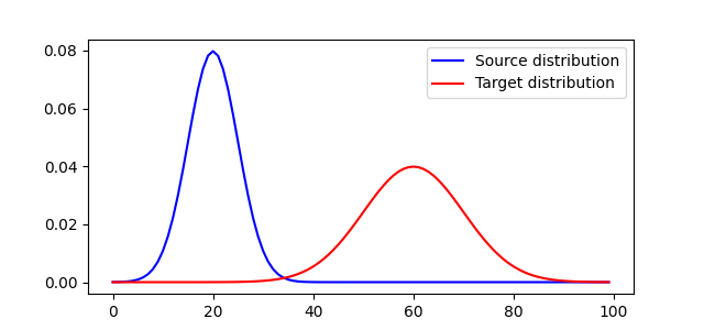
<matplotlib.legend.Legend object at 0x7f590d9f53f0>

pl.figure(2, figsize=(5, 5))
ot.plot.plot1D_mat(a, b, M, "Cost matrix M")

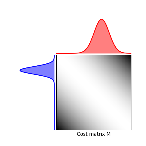
(<Axes: >, <Axes: >, <Axes: >)

解决EMD

# use fast 1D solver
G0 = ot.emd_1d(x, x, a, b)

# Equivalent to
# G0 = ot.emd(a, b, M)

pl.figure(3, figsize=(5, 5))
ot.plot.plot1D_mat(a, b, G0, "OT matrix G0")

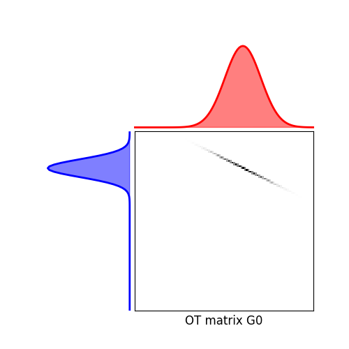
(<Axes: >, <Axes: >, <Axes: >)

解决Sinkhorn

lambd = 1e-3
Gs = ot.sinkhorn(a, b, M, lambd, verbose=True)

pl.figure(4, figsize=(5, 5))
ot.plot.plot1D_mat(a, b, Gs, "OT matrix Sinkhorn")

pl.show()

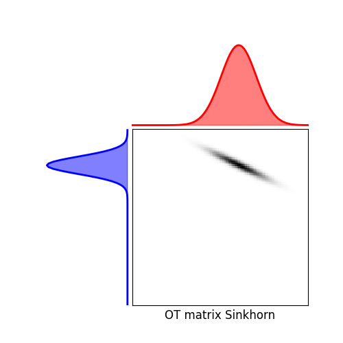
It.  |Err
-------------------
    0|2.861463e-01|
   10|1.860154e-01|
   20|8.144529e-02|
   30|3.130143e-02|
   40|1.178815e-02|
   50|4.426078e-03|
   60|1.661047e-03|
   70|6.233110e-04|
   80|2.338932e-04|
   90|8.776627e-05|
  100|3.293340e-05|
  110|1.235791e-05|
  120|4.637176e-06|
  130|1.740051e-06|
  140|6.529356e-07|
  150|2.450071e-07|
  160|9.193632e-08|
  170|3.449812e-08|
  180|1.294505e-08|
  190|4.857493e-09|
It.  |Err
-------------------
  200|1.822723e-09|