一维的OT距离

展示如何计算多个Wasserstein和Sinkhorn，使用两种不同的基础度量，并绘制它们在不同分布下的值。

# Author: Remi Flamary <remi.flamary@unice.fr>
#
# License: MIT License

# sphinx_gallery_thumbnail_number = 2

import numpy as np
import matplotlib.pylab as pl
import ot
from ot.datasets import make_1D_gauss as gauss

生成数据

n = 100  # nb bins
n_target = 20  # nb target distributions


# bin positions
x = np.arange(n, dtype=np.float64)

lst_m = np.linspace(20, 90, n_target)

# Gaussian distributions
a = gauss(n, m=20, s=5)  # m= mean, s= std

B = np.zeros((n, n_target))

for i, m in enumerate(lst_m):
    B[:, i] = gauss(n, m=m, s=5)

# loss matrix and normalization
M = ot.dist(x.reshape((n, 1)), x.reshape((n, 1)), "euclidean")
M /= M.max() * 0.1
M2 = ot.dist(x.reshape((n, 1)), x.reshape((n, 1)), "sqeuclidean")
M2 /= M2.max() * 0.1

绘制数据

pl.figure(1)
pl.subplot(2, 1, 1)
pl.plot(x, a, "r", label="Source distribution")
pl.title("Source distribution")
pl.subplot(2, 1, 2)
for i in range(n_target):
    pl.plot(x, B[:, i], "b", alpha=i / n_target)
pl.plot(x, B[:, -1], "b", label="Target distributions")
pl.title("Target distributions")
pl.tight_layout()

计算不同损失的EMD

d_emd = ot.emd2(a, B, M)  # direct computation of OT loss
d_emd2 = ot.emd2(a, B, M2)  # direct computation of OT loss with metric M2
d_tv = [np.sum(abs(a - B[:, i])) for i in range(n_target)]

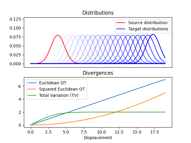
pl.figure(2)
pl.subplot(2, 1, 1)
pl.plot(x, a, "r", label="Source distribution")
pl.title("Distributions")
for i in range(n_target):
    pl.plot(x, B[:, i], "b", alpha=i / n_target)
pl.plot(x, B[:, -1], "b", label="Target distributions")
pl.ylim((-0.01, 0.13))
pl.xticks(())
pl.legend()
pl.subplot(2, 1, 2)
pl.plot(d_emd, label="Euclidean OT")
pl.plot(d_emd2, label="Squared Euclidean OT")
pl.plot(d_tv, label="Total Variation (TV)")
# pl.xlim((-7,23))
pl.xlabel("Displacement")
pl.title("Divergences")
pl.legend()

<matplotlib.legend.Legend object at 0x7f590d5b5960>

计算不同损失的Sinkhorn

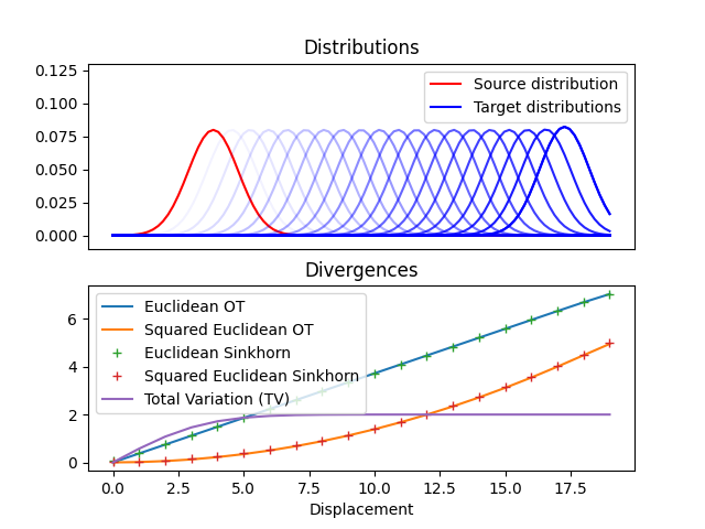
reg = 1e-1
d_sinkhorn = ot.sinkhorn2(a, B, M, reg)
d_sinkhorn2 = ot.sinkhorn2(a, B, M2, reg)

pl.figure(3)
pl.clf()

pl.subplot(2, 1, 1)
pl.plot(x, a, "r", label="Source distribution")
pl.title("Distributions")
for i in range(n_target):
    pl.plot(x, B[:, i], "b", alpha=i / n_target)
pl.plot(x, B[:, -1], "b", label="Target distributions")
pl.ylim((-0.01, 0.13))
pl.xticks(())
pl.legend()
pl.subplot(2, 1, 2)
pl.plot(d_emd, label="Euclidean OT")
pl.plot(d_emd2, label="Squared Euclidean OT")
pl.plot(d_sinkhorn, "+", label="Euclidean Sinkhorn")
pl.plot(d_sinkhorn2, "+", label="Squared Euclidean Sinkhorn")
pl.plot(d_tv, label="Total Variation (TV)")
# pl.xlim((-7,23))
pl.xlabel("Displacement")
pl.title("Divergences")
pl.legend()
pl.show()