注意

This page was generated from gallery/plot_clip.ipynb.

Interactive online version:

使用GeoPandas剪切矢量数据

了解如何使用GeoPandas将几何图形裁剪到多边形几何图形的边界。

下面的示例向您展示如何将一组矢量几何图形裁剪到另一个矢量对象的空间范围/形状。两组几何图形必须使用GeoPandas作为GeoDataFrames打开，并且必须在同一坐标参考系统（CRS）中，以便GeoPandas中的clip函数能够工作。

此示例使用来自 geodatasets 'geoda.chicago-health' 和 'geoda.groceries' 的示例数据，以及使用 shapely 制作的自定义矩形几何图形，随后转换为 GeoDataFrame。

注意

待裁剪的对象将被裁剪到裁剪对象的全部范围。如果裁剪对象中有多个多边形，输入数据将被裁剪到裁剪对象中所有多边形的总边界。

导入包

首先，导入所需的包。

import matplotlib.pyplot as plt
import geopandas
from shapely.geometry import box
import geodatasets

获取或创建示例数据

下面，示例的 GeoPandas 数据被导入并作为 GeoDataFrame 打开。此外，使用 shapely 创建一个多边形，然后将其转换为与 GeoPandas chicago 数据集具有相同 CRS 的 GeoDataFrame。

chicago = geopandas.read_file(geodatasets.get_path("geoda.chicago_commpop"))
groceries = geopandas.read_file(geodatasets.get_path("geoda.groceries")).to_crs(chicago.crs)

# Create a subset of the chicago data that is just the South American continent
near_west_side = chicago[chicago["community"] == "NEAR WEST SIDE"]

# Create a custom polygon
polygon = box(-87.8, 41.90, -87.5, 42)
poly_gdf = geopandas.GeoDataFrame([1], geometry=[polygon], crs=chicago.crs)

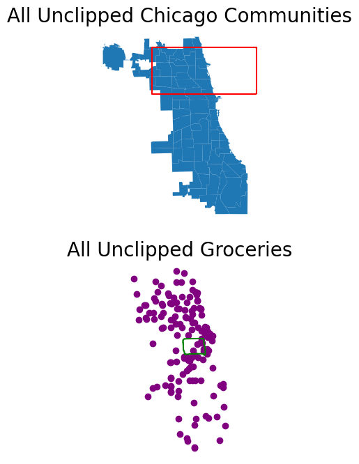
绘制未裁剪的数据

fig, (ax1, ax2) = plt.subplots(2, 1, figsize=(12, 8))
chicago.plot(ax=ax1)
poly_gdf.boundary.plot(ax=ax1, color="red")
near_west_side.boundary.plot(ax=ax2, color="green")
groceries.plot(ax=ax2, color="purple")
ax1.set_title("All Unclipped Chicago Communities", fontsize=20)
ax2.set_title("All Unclipped Groceries", fontsize=20)
ax1.set_axis_off()
ax2.set_axis_off()
plt.show()

裁剪数据

您调用 clip 的对象是将要被裁剪的对象。您传递的对象是裁剪范围。返回的输出将是一个新的裁剪后的 GeoDataframe。当您进行裁剪时，所有返回几何图形的属性将被保留。

注意

请记住，为了使用clip方法，数据必须在相同的坐标参考系统（CRS）中。如果数据不在相同的CRS中，请务必使用GeoPandas GeoDataFrame.to_crs方法，以确保两个数据集在相同的坐标参考系统中。

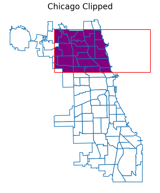
裁剪芝加哥数据

chicago_clipped = chicago.clip(polygon)

# Plot the clipped data
# The plot below shows the results of the clip function applied to the chicago
# sphinx_gallery_thumbnail_number = 2
fig, ax = plt.subplots(figsize=(12, 8))
chicago_clipped.plot(ax=ax, color="purple")
chicago.boundary.plot(ax=ax)
poly_gdf.boundary.plot(ax=ax, color="red")
ax.set_title("Chicago Clipped", fontsize=20)
ax.set_axis_off()
plt.show()

注意

出于历史原因，clip 方法也可作为顶级函数 geopandas.clip 使用。建议使用该方法，因为该函数在未来可能会被弃用。

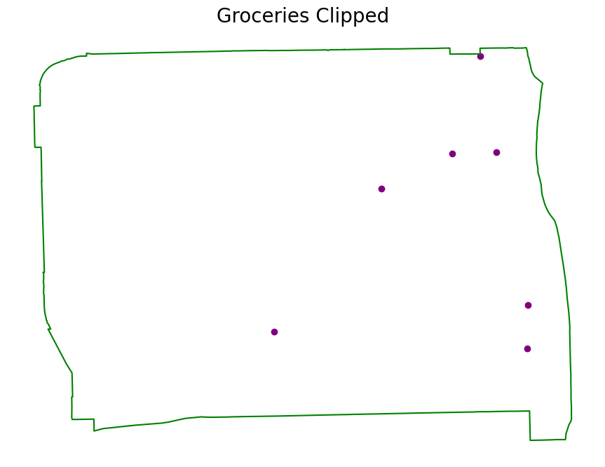
裁剪杂货数据

groceries_clipped = groceries.clip(near_west_side)

# Plot the clipped data
# The plot below shows the results of the clip function applied to the capital cities
fig, ax = plt.subplots(figsize=(12, 8))
groceries_clipped.plot(ax=ax, color="purple")
near_west_side.boundary.plot(ax=ax, color="green")
ax.set_title("Groceries Clipped", fontsize=20)
ax.set_axis_off()
plt.show()